Reading a Real Transformer: DistilBERT Up Close

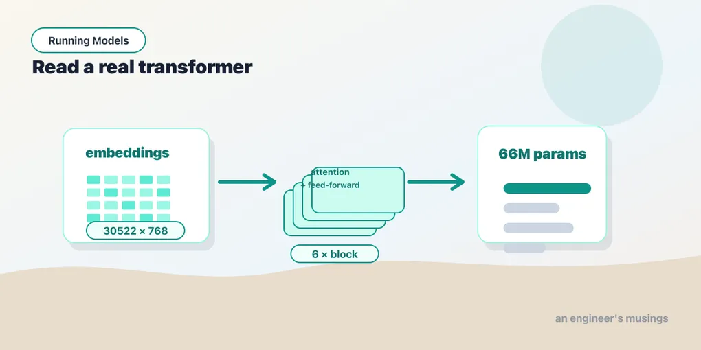
The last chapter ended with the transformer block on paper — an embedding lookup, then self-attention, a feed-forward network, a couple of norms, stacked. Now we open a real one. DistilBERT is a genuine, pretrained language model with about sixty-six million numbers inside, and it is the model behind the sentiment three-liner you have run twice. This is the text-world twin of chapter 12, where we cracked open ResNet: same move, same skills, same payoff. We’re going to print it, read the tree, and find nothing in it but the pieces you already named.

▶ Open the companion notebook in Colab

Run against: PyTorch 2.2.2 and transformers 4.57.6 on CPU (macOS); where transformers 5.x behaves differently the text says so, from its source.

The pieces you’ll see

A transformer’s printout is longer than ResNet’s, but it’s built from a shorter list of parts — and you met all of them in the last chapter:

• Embedding — a lookup table that turns each token ID into a vector. There’s one row per word in the vocabulary; “give me token 2,054” just reads off row 2,054. This is the entry point of every language model, the text equivalent of ResNet’s first Conv2d.
• MultiHeadSelfAttention — the new idea from chapter 13: every word looks at every other word and gathers what’s relevant.
• FFN — the feed-forward network, the small MLP that processes each position after attention.
• LayerNorm — the steadying supporting cast, same as in ResNet. Read right past it on a first pass.

Look up the word, let the words look at each other, think a little, repeat — that carries you through the whole model.

Loading DistilBERT and reading it

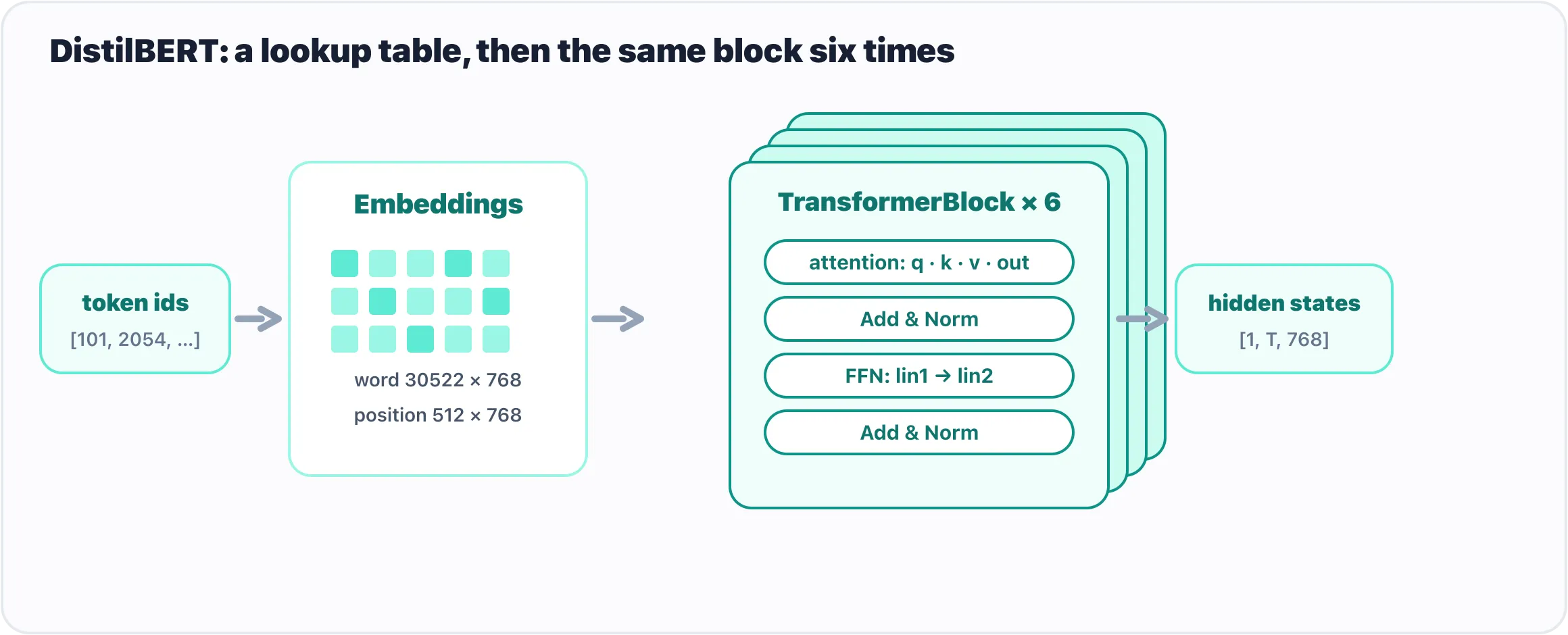
DistilBERT is an embeddings table feeding six identical transformer blocks.

We’ll grab DistilBERT and its pretrained weights straight from the Hugging Face Hub. (The transformers library isn’t in Colab by default, so install it once first.)

!pip install -q transformers

from transformers import AutoModel

model = AutoModel.from_pretrained("distilbert-base-uncased")

AutoModel.from_pretrained downloads the architecture and its trained weights (a state dict, in the .safetensors format chapter 11 mentioned) and hands you the assembled model — the text-world counterpart of resnet50(weights=...). The first run downloads; after that it’s cached. The bare name distilbert-base-uncased still works because the Hub redirects it; its canonical address is distilbert/distilbert-base-uncased. Now do the exact thing you did with ResNet — just print it:

print(model)

You’ll get a long, indented outline. Don’t read every line; read the shape of it. The top says DistilBertModel(, and nested inside are three things:

DistilBertModel(
  (embeddings): Embeddings(
    (word_embeddings): Embedding(30522, 768, padding_idx=0)
    (position_embeddings): Embedding(512, 768)
    (LayerNorm): LayerNorm((768,), ...)
  )
  (transformer): Transformer(
    (layer): ModuleList(
      (0-5): 6 x TransformerBlock(
        (attention): MultiHeadSelfAttention(
          (q_lin): Linear(in_features=768, out_features=768, bias=True)
          (k_lin): Linear(in_features=768, out_features=768, bias=True)
          (v_lin): Linear(in_features=768, out_features=768, bias=True)
          (out_lin): Linear(in_features=768, out_features=768, bias=True)
        )
        (sa_layer_norm): LayerNorm((768,), ...)
        (ffn): FFN(
          (lin1): Linear(in_features=768, out_features=3072, bias=True)
          (lin2): Linear(in_features=3072, out_features=768, bias=True)
        )
        (output_layer_norm): LayerNorm((768,), ...)
      )
    )
  )
)

That indentation is the tree, the same kind ResNet had. Read it top to bottom:

• embeddings turns token IDs into 768-number vectors. Embedding(30522, 768) is the vocabulary table — 30,522 known tokens, each a row of 768 numbers — plus a small position_embeddings table so the model knows word order (the thing a plain Linear couldn’t track).
• transformer is the stack. (0-5): 6 x TransformerBlock is PyTorch telling you there are six identical blocks in a row. And inside each block? Exactly chapter 13’s anatomy: an attention (here you can even see its four Linears — the query, key, value, and output projections that make attention work), a LayerNorm, an ffn with its two Linears, and another LayerNorm.

That’s the whole model: a lookup table, then the same block six times. The printout is just its table of contents — and you read it knowing no math.

Counting the parameters

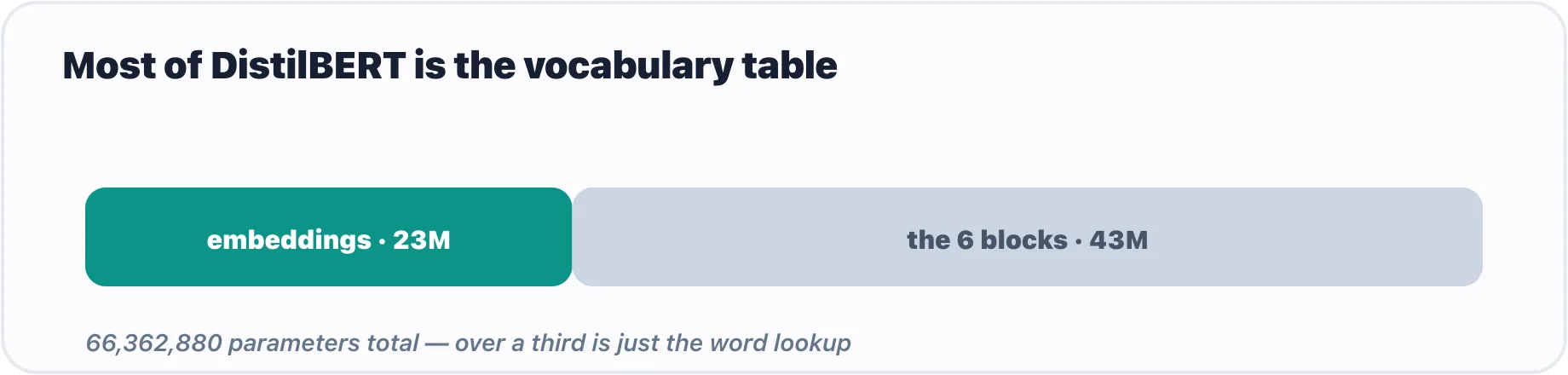
Over a third of DistilBERT’s 66M parameters live in the word-embedding table.

The parameters are the actual learned numbers — the weights tuned during training. Count them with the same one-liner you ran on ResNet:

total = sum(p.numel() for p in model.parameters())
print(f"{total:,} parameters")   # 66,362,880 parameters

About 66 million numbers. That’s why it’s called DistilBERT — it’s a distilled, slimmed-down BERT, built to be small and fast while keeping most of the ability. (Full BERT is more than twice the size; today’s large language models are a thousandfold bigger still. DistilBERT is the friendly one.)

Here’s a detail worth pausing on. Look where those numbers live:

for name, p in list(model.named_parameters())[:4]:
    print(name, tuple(p.shape))

embeddings.word_embeddings.weight (30522, 768)
embeddings.position_embeddings.weight (512, 768)
transformer.layer.0.attention.q_lin.weight (768, 768)
transformer.layer.0.attention.q_lin.bias (768,)

That first line alone — the word-embeddings table — is 30,522 × 768, which is over 23 million numbers, more than a third of the whole model. A huge share of a language model is just the dictionary: a learned vector for every token it knows. The same naming logic as ResNet applies, too — transformer.layer.0.attention.q_lin.weight is “the query projection’s weight, in attention, in block 0.” It’s a path through the tree you just printed.

Backbone or head: what AutoModel actually gave you

This is the most useful thing in Part II for someone who only wants to run models, so it gets its own section rather than a gotcha. What you printed is the backbone: embeddings and six blocks, and nothing after them. Feed it a sentence and what comes out is a tensor of shape [1, tokens, 768] — one 768-number vector per token, the “hidden states” of chapter 5 — not a label. The sentiment three-liner runs this exact backbone plus one more layer: a small classification head on top that turns the summary vector into two scores. That head is what the For… in AutoModelForSequenceClassification means.

from transformers import AutoModelForSequenceClassification

clf = AutoModelForSequenceClassification.from_pretrained(
    "distilbert/distilbert-base-uncased-finetuned-sst-2-english"
)
print(clf.pre_classifier)    # Linear(in_features=768, out_features=768, bias=True)
print(clf.classifier)        # Linear(in_features=768, out_features=2, bias=True)

Same backbone, then a small head — a 768-to-768 Linear, a dropout, and a final 768-to-2 Linear — and two outputs: the [1, 2] logits chapter 5 previewed. So the rule for the rest of the book: AutoModel when you want the vectors (embeddings, chapter 19), AutoModelFor<task> when you want an answer (classification in chapter 17, generation in chapter 22). The model card tells you which heads a checkpoint was trained with; asking for a head it never had gives you a freshly initialised, random one, and a warning you should not ignore.

Gotchas

• print(model) shows structure, not the weights. It lists layers and sizes — it does not dump sixty-six million numbers. To touch values you go through .parameters() or .named_parameters(), exactly as with ResNet.
• for p in model.parameters() will flood your screen. A real transformer has hundreds of parameter tensors. Always slice — list(model.named_parameters())[:4] — when you just want a peek.
• The vocabulary is most of the model. It surprises people that the “intelligence” layers are a minority of the parameters and the embedding table is so large. That’s normal for smaller models like this one.
• The depth is the only thing that’s new. Six identical blocks read longer than ResNet’s printout, but it’s the same short list of parts repeated. If it looks intimidating, it’s the length, not the kind of thing in it.

What’s next

The box is glass here too. DistilBERT is an nn.Module — an embedding table feeding six copies of the attention-and-feed-forward block from the last chapter — and reading it took nothing you didn’t already have. You’ve now done for transformers exactly what you did for vision models: met the idea, then opened a real one, and learned to tell a backbone from a head.

One more thing closes Part II, and it is the most practical use of everything in it. Every model so far arrived through a library that knew where its weights were. The next chapter loads weights that are not on the Hub at all — a state dict from a plain URL, into an architecture you build yourself — and puts a face on it.

Next: Loading Weights That Aren’t on the Hub: A Live Digit Reader.