Series: Practical PyTorch · II (Phase II) — Part 2 of 9

Part 1 gave you the intuition: a model learns by guessing, measuring how wrong it was, and nudging its numbers in the direction that makes it less wrong — over and over, until the guesses are good. That’s the whole story. This post turns that story into code, because the remarkable thing about PyTorch is that the entire mechanism fits in about five lines, and once you’ve seen those five lines work on a toy example, every training script you ever read afterward stops being mysterious.

We’ll fit a tiny model to a handful of made-up numbers, print the loss as it falls, and pull apart what each line is doing. It trains in well under a second on a plain CPU — no GPU, no dataset download, nothing to install beyond PyTorch.

▶ Open the companion notebook in Colab

A tiny model and some toy data

Let’s give the model the easiest possible job: learn the rule y = 2x + 1. We won’t tell it that rule — we’ll hand it some (x, y) pairs that follow it and let it figure out the 2 and the 1 on its own. If it can recover those, learning happened.

import torch
import torch.nn as nn

# Toy data: y = 2x + 1, with a little noise so it's not too easy.
x = torch.linspace(-1, 1, 100).unsqueeze(1)      # shape [100, 1]
y = 2 * x + 1 + 0.1 * torch.randn_like(x)        # shape [100, 1]

model = nn.Linear(1, 1)   # one input, one output: learns a slope and a bias

nn.Linear(1, 1) is the smallest real model there is — it holds exactly two numbers, a slope (weight) and an intercept (bias), and computes slope * x + bias. They start out random, so right now the model is confidently wrong. Our job is to fix that.

The unsqueeze(1) turns a flat list of 100 numbers into a column of shape [100, 1], because PyTorch layers expect a batch of inputs where each input is itself a little vector — even when that vector has length one.

The loss function and the optimizer

Two more objects before the loop. The loss function scores how wrong the model is, and the optimizer knows how to adjust the model’s numbers to lower that score.

loss_fn = nn.MSELoss()                                 # for predicting numbers
optimizer = torch.optim.SGD(model.parameters(), lr=0.1)  # the "nudger"

nn.MSELoss is mean squared error — it takes the gap between each prediction and the true value, squares it (so big misses hurt disproportionately, and sign doesn’t matter), and averages. It’s the standard choice when your model predicts a continuous number. When you’re predicting categories instead — cat vs. dog, spam vs. not — you’d reach for nn.CrossEntropyLoss, which we’ll meet in a later post.

torch.optim.SGD is stochastic gradient descent, the plainest optimizer there is. You hand it model.parameters() so it knows which numbers it’s allowed to touch, and a learning rate (lr) that controls how big each nudge is. Adam (torch.optim.Adam) is a fancier, more forgiving optimizer that most people default to for real work; SGD is perfect for seeing the mechanism clearly.

The loop, one line at a time

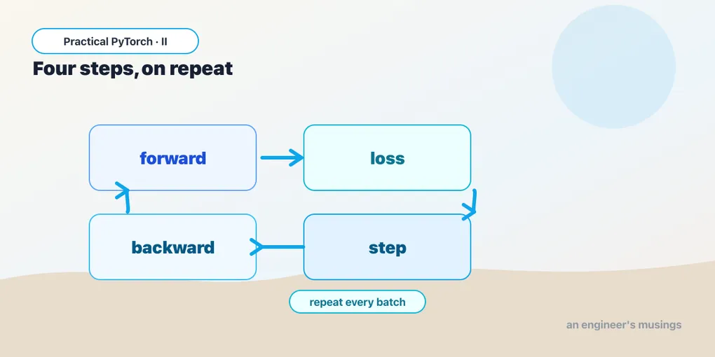
Here it is — the canonical PyTorch training loop. Five steps, repeated for a number of epochs (one epoch = one pass over the data):

for epoch in range(100):
    preds = model(x)              # 1. forward:   guess
    loss = loss_fn(preds, y)      # 2. loss:      how wrong?

    optimizer.zero_grad()         # 3. clear old gradients
    loss.backward()               # 4. backward:  work out the nudge
    optimizer.step()              # 5. step:      apply the nudge

    if epoch % 10 == 0:
        print(f"epoch {epoch:3d}  loss {loss.item():.4f}")

Let’s take the five steps in turn, because each one is a real concept and they’re the same five in every training script you’ll ever see.

1. Forward — preds = model(x). The model takes the inputs and produces predictions. With random starting numbers these are garbage, and that’s fine. This is exactly the “run a model” pattern from Phase I; training just does it in a loop.

2. Loss — loss = loss_fn(preds, y). Compare the guesses to the truth and collapse the whole mess into a single number. Lower is better. This number is the thing the rest of the loop is trying to drive down.

3. Zero the gradients — optimizer.zero_grad(). This is the one that trips everybody up, so hold that thought — there’s a section on it below. For now: it wipes the slate clean before we compute fresh adjustments.

4. Backward — loss.backward(). This is autograd, the part Phase I told you to ignore, finally earning its keep. PyTorch has been quietly recording every operation that led to loss. Calling .backward() runs that recording in reverse and works out, for every parameter, which direction and how much it should change to reduce the loss. Those answers are the gradients, and PyTorch tucks them onto each parameter. You never compute a derivative by hand — that’s the entire point of autograd.

5. Step — optimizer.step(). The optimizer reads the gradients autograd just computed and nudges each parameter accordingly, scaled by the learning rate. This is the line where the model actually changes. Everything before it was measurement and planning; this is the move.

Run that, do it a hundred times, and the model walks itself from random nonsense toward y = 2x + 1.

Watch the loss drop

When you run the loop, you’ll see something like this:

epoch   0  loss 3.8421
epoch  10  loss 0.4773
epoch  20  loss 0.0931
epoch  30  loss 0.0291
epoch  40  loss 0.0144
...
epoch  90  loss 0.0102

That falling number is learning — there’s no other magic. And because our model only holds two numbers, we can check that it found the right ones:

print("weight:", model.weight.item())   # should be near 2.0
print("bias:  ", model.bias.item())     # should be near 1.0

You’ll get something like 1.98 and 1.01 — not exact, because we added noise to the data, but the model recovered the rule we never told it. That’s the satisfying moment: it figured out the slope and intercept purely from examples.

Gotchas

A handful of mistakes account for most “why isn’t my model learning?” confusion. Forewarned is forearmed.

• Forgetting optimizer.zero_grad(). Gradients in PyTorch accumulate — each .backward() adds to whatever is already stored rather than replacing it. Skip the zeroing and you’re stepping on the sum of this epoch’s gradient and every previous one, which sends training haywire. If your loss explodes or refuses to settle, this is the first thing to check. (The accumulation behavior is occasionally useful on purpose, for very large batches, but until you need that, always zero.)
• The wrong loss for the task. MSELoss is for predicting numbers; CrossEntropyLoss is for predicting which category something belongs to. Use MSE on a classification problem and the model will technically “train” while learning something nonsensical. Match the loss to the job.
• A learning rate that’s wrong by a lot. Too high and the nudges overshoot — the loss bounces around or blows up to nan. Too low and it crawls, taking thousands of epochs to get anywhere. lr is the first knob to turn when training misbehaves; try changing it by factors of ten (0.001, 0.01, 0.1) rather than tiny tweaks.
• Comparing preds and y with mismatched shapes. If preds is [100, 1] and y is [100], some loss functions will silently broadcast them into a [100, 100] mess and report a meaningless loss. Keep their shapes identical; that’s why we used unsqueeze above.
• Forgetting train vs. eval mode. Our toy model doesn’t care, but real models contain layers (dropout, batch-norm) that behave differently while learning versus while being used. The habit to build now: call model.train() before your training loop and model.eval() before you evaluate or predict. It costs nothing here and saves a baffling bug later.
• Measuring gradients without requires_grad. Model parameters created by nn.Linear already have requires_grad=True, which is what lets autograd track them — you don’t set it yourself for normal models. Just know that’s the flag doing the bookkeeping, and that wrapping prediction code in with torch.no_grad(): turns the tracking off when you only want answers, not learning.

What’s next

You’ve now seen the engine Phase I told you to ignore, running in the open: forward, loss, zero_grad, backward, step. Every training script — from a two-parameter line-fitter to a billion-parameter language model — is this same loop with bigger models and more data wrapped around it.

And “more data” is the next problem. Feeding 100 toy numbers in one go is easy; feeding millions of images in shuffled, batched chunks without running out of memory needs real tooling. That’s what PyTorch’s Dataset and DataLoader are for.

Next: Part 3 — Datasets and DataLoaders, how to feed a training loop without melting your machine.

---

Target keyword(s): pytorch training loop, loss backward optimizer step, pytorch training loop for beginners.