Series: Practical PyTorch · II (Phase II) — Part 1 of 9

Phase I made one promise over and over: you don’t need the math to run a model. That was true, and it still is. But now we’re crossing a line. Phase II is about changing models — fine-tuning them on your own data so they do something the off-the-shelf version couldn’t. And to do that, you finally need a mental model of how a model learns in the first place.

Here’s the deal I’ll make with you: no calculus, no derivatives, no chain rule. Just the intuition — the handful of ideas that, once they click, make training stop feeling like magic. There’s a tiny bit of code at the end, but this post is mostly about building the picture in your head.

▶ Open the companion notebook in Colab

The whole idea: learning by being wrong

A neural network is, at its core, a big pile of numbers called weights. When you feed it an input, those numbers get multiplied and added together to produce an output — a prediction. At the start, the weights are random, so the predictions are garbage. A fresh model shown a photo of a cat will confidently guess “fire truck.”

So how does it get good? Not by being told the right answer and memorizing it. It gets good through a loop that’s almost insultingly simple:

1. The model makes a prediction.
2. We measure how wrong it was — as a single number.
3. We work out which way to nudge each weight to make that number a little smaller.
4. We nudge — gently.
5. Repeat. Thousands of times. Sometimes millions.

That’s it. That’s training. Every weight starts random and bad, and the loop slowly bends them toward “less wrong.” Do it enough times on enough examples and “less wrong” quietly becomes “actually pretty good.” Let’s give the pieces their real names.

Loss: one number for “how wrong”

The loss is a single number that says how badly the model did on an example (or a batch of examples). Big loss means the prediction was way off. Loss near zero means the prediction was nearly perfect.

The whole goal of training is to make this number go down. That’s the entire game — everything else is in service of shrinking the loss. The specific recipe for computing it (mean squared error, cross-entropy, and friends) doesn’t matter much to you right now; what matters is the idea: loss is the score, and lower is better.

Gradient: which way to nudge

Now the magic question: we have a loss, and we want it smaller — so which way do we move each weight? Up a touch? Down a lot?

The answer is the gradient. For every weight in the model, the gradient tells you two things: the direction to nudge that weight to reduce the loss, and how much moving it would help. Think of it as an arrow attached to each weight saying “push me this way, this hard, and the loss goes down.”

That’s the entire intuition. No derivatives, no equations — just which direction, and how much, for each weight. The gradient is the downhill direction for the loss.

Optimizer: the thing that actually does the nudging

The gradient tells you where downhill is. The optimizer is the thing that takes the step. It looks at the gradient for every weight and updates them all, nudging each one in its downhill direction.

You’ll meet two by name:

• SGD (Stochastic Gradient Descent) — the classic. Plain, dependable, takes a straightforward step downhill.
• Adam — the popular modern default. Smarter about how big a step to take for each weight, and usually trains faster with less fiddling. When in doubt, people reach for Adam.

You don’t implement these. You pick one, hand it the model’s weights, and it does the stepping for you — one line of code, which you’ll see in Part 2.

Learning rate: how big each nudge is

The gradient says which way and the optimizer takes the step, but how big is that step? That’s the learning rate — a single dial you set, and arguably the most important one in all of training.

• Too big, and you overshoot. You leap past the bottom and bounce around, or fly off entirely. The loss jumps around or explodes instead of settling.
• Too small, and you crawl. Training technically works but takes forever, inching downhill so slowly you run out of patience (or budget).

Getting the learning rate into the right ballpark is most of what “tuning” a model feels like in practice. There’s no universal correct value — but there’s a wide band of “good enough,” and you learn to find it.

Epoch: one full pass over the data

You don’t show the model your dataset once and call it done. You show it the whole thing, over and over. One complete pass through all your training data is an epoch.

Training for, say, 3 epochs means the model sees every example three times, nudging its weights a little on each. More epochs means more chances to improve — up to a point, after which it starts memorizing your specific examples instead of learning the general pattern (we’ll deal with that in a later post). For now: an epoch is one lap around the dataset.

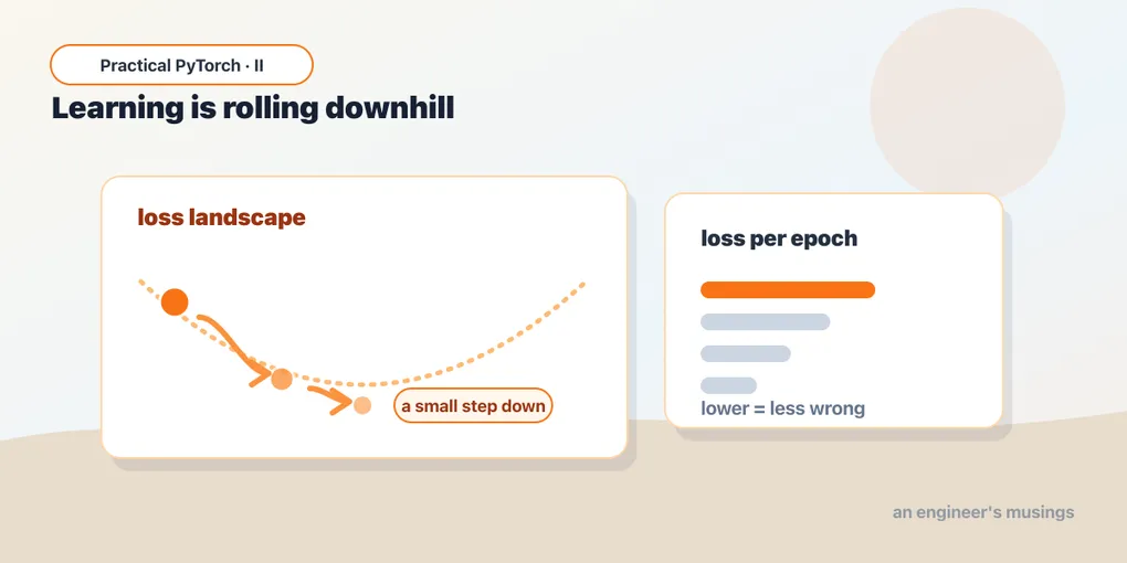
The foggy-hill picture

Here’s the analogy to hang all of this on. Imagine you’re standing on a hillside in thick fog, and you want to reach the lowest point in the valley. You can’t see the bottom — the fog is too thick. But you can feel the ground right under your feet.

So you do the only sensible thing: you feel which way the ground slopes downhill, and you take a step that way. Then you feel again, and step again. Step by step, you descend — never seeing the whole landscape, just always moving in the locally-downhill direction.

Map it back:

• The height where you’re standing is the loss — you want to get low.
• The slope under your feet is the gradient — which way is downhill.
• Taking a step is the optimizer doing its update.
• The size of your step is the learning rate — giant leaps overshoot the valley; tiny shuffles take all day.
• Walking the entire hill once, considering every patch of ground, is an epoch.

It’s the children’s game of hot-and-cold, played by a machine, on a landscape with millions of dimensions, a few thousand times a second. The model never sees the whole map. It just keeps feeling for downhill and stepping. And that’s enough.

Where autograd fits

Remember in Phase I, when I kept saying you never touch autograd? That you could drive the whole car without opening the hood? This is the part of the engine I was pointing at.

Computing the gradient — the downhill direction for every single weight at once — is the genuinely hard math. A modern model has millions or billions of weights, and figuring out the nudge for each one would be hopeless by hand. Autograd is the machinery that computes all those gradients for you, automatically. You define the model and the loss; autograd works out the arrows.

That’s why Phase I could skip it entirely: when you’re only running a model, no weights are changing, so no gradients are needed and autograd just sits there. The moment you start training, autograd wakes up and does the heaviest lifting in the whole process — silently, behind one method call you’ll meet next post. You still don’t have to understand how it computes the gradients. You just have to know that’s its job.

Gotchas

• Learning rate is the dial that bites first. If training “isn’t working,” nine times out of ten the learning rate is too high (loss explodes or bounces) or too low (loss barely moves). Adjust it before you suspect anything fancier.
• “Training” and “running” are different modes. Running a model is read-only — weights stay frozen, you just get predictions. Training changes the weights. Phase I was all running; Phase II is training. Don’t expect a model to improve just because you used it a lot — it learns only inside the training loop.
• Loss going down is good; loss going up is a flashing red light. A healthy run shows loss generally drifting downward. If it climbs or swings wildly, stop and look at your learning rate (and your data) before letting it burn more time.
• It’s not magic, it’s a lot of small corrections. No single step makes the model smart. The intelligence is emergent from thousands of tiny “less wrong” nudges. If that feels anticlimactic — good, that’s the honest picture.
• Lower loss isn’t the same as a better model. A model can drive its loss to near-zero by memorizing the training examples and still be useless on anything new. We’ll separate “low loss” from “actually good” when we get to evaluation.
• The model only learns what’s in the data. The loop faithfully optimizes toward whatever your examples reward. Biased or sloppy data produces a confidently biased or sloppy model — the math has no opinion about whether your labels were any good.

What’s next

You now have the mental model: predict, measure the loss, find the downhill gradient, let the optimizer take a step sized by the learning rate, and repeat for a few epochs. That’s the loop that turns a pile of random numbers into something useful.

Next we write it down in actual PyTorch — the few lines that run that loop, with autograd quietly handling the hard part.

Next: Part 2 — The Training Loop, in Code, where the foggy-hill walk becomes about a dozen lines you can run.

---

Target keyword(s): how neural networks learn, training intuition, pytorch fine-tuning for beginners.