Series: Practical PyTorch · I (Phase I) — Part 6 of 9

In Part 4 you ran a pretrained model end to end, and it took maybe ten lines: load the model, load its preprocessing, shape the input just so, run it, then turn the raw numbers back into something a human can read. It worked, and it was worth doing once by hand so the machinery isn’t a mystery. But ten lines every time you want to classify a sentence is a tax nobody should pay. This post is about the shortcut, and it’s a big one.

▶ Open the companion notebook in Colab

The shortcut is pipeline, from the transformers library. It’s the single highest-leverage tool in this whole series. Most “I just want to run a model” tasks collapse from ten lines to three, and the three lines read like plain intent.

Install it, then run a model

transformers isn’t in Colab by default, so install it once per session:

!pip install -q transformers

Now the famous three lines. The first thing nearly everyone runs is sentiment analysis — hand it text, get back a verdict:

from transformers import pipeline

clf = pipeline("sentiment-analysis")
print(clf("I can't believe how easy this was."))
# [{'label': 'POSITIVE', 'score': 0.9998}]

That’s it. You didn’t pick a model, you didn’t write any preprocessing, you didn’t decode anything. You named a task ("sentiment-analysis"), and pipeline did the rest. It even pulled a sensible default model down for you on that first call, picked the matching tokenizer, and wired the whole thing together. The score, by the way, is the model’s confidence in the label it chose; 0.9998 means it’s quite sure that sentence is positive.

It’s the Part 5 recipe, automated

Here’s the thing worth internalizing, because it’s why pipeline isn’t magic and won’t leave gaps in your understanding: it’s doing exactly the steps you did by hand in Part 5, just hidden behind one callable.

Remember the shape of that work — preprocess, forward, postprocess:

1. Preprocess — take your raw input (a string, an image, an audio clip) and turn it into tensors the model expects. For text that’s tokenization; for images it’s resizing and normalizing.
2. Forward — run those tensors through the model and get raw output (logits, basically: unscaled scores).
3. Postprocess — turn that raw output back into something useful: a label, a probability, a sentence.

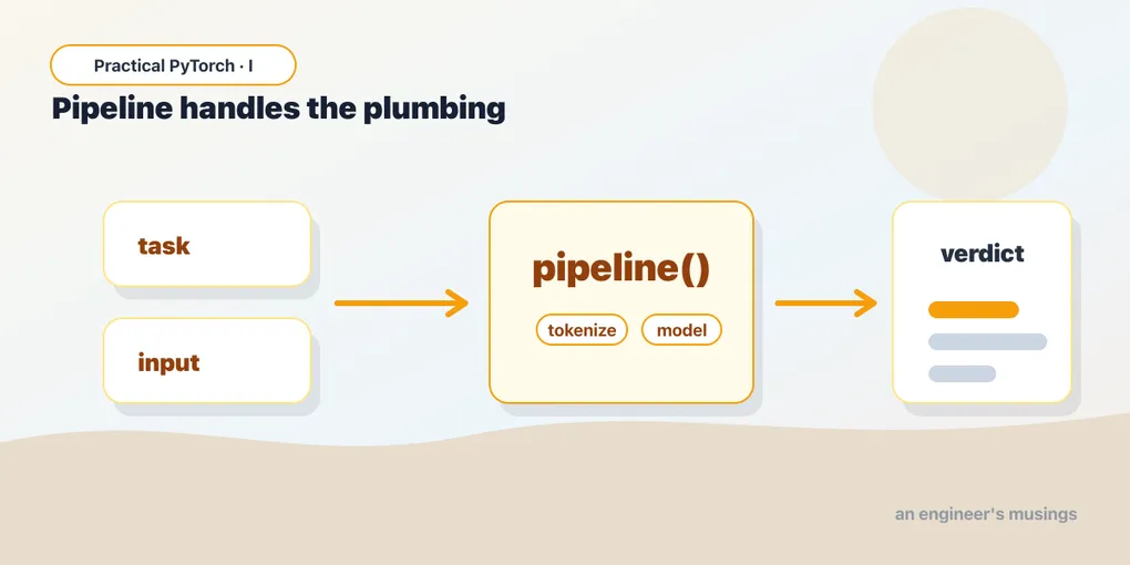
pipeline bundles all three. When you call clf("..."), it tokenizes your string, runs the model, and converts the logits into that tidy {'label': 'POSITIVE', 'score': 0.9998} for you. Same recipe, same model, none of the boilerplate. You’re not skipping the steps — you’ve just stopped typing them.

A tour of tasks

The real reason pipeline is the workhorse: the same three-line pattern works across wildly different jobs. You change the task name, and occasionally the arguments, and that’s the whole story. Text in, text out; image in, label out; audio in, transcript out. Here’s a quick tour, and as you read it, watch how little actually changes between examples.

Summarization — feed it a wall of text, get back a short version:

summarize = pipeline("summarization")
print(summarize(long_article, max_length=60, min_length=20))
# [{'summary_text': '...'}]

max_length and min_length are token budgets for the summary, not strict character counts, so treat them as rough dials rather than exact limits.

Zero-shot classification — sort text into categories you invent on the spot, with no training:

route = pipeline("zero-shot-classification")
print(route(
    "My card was charged twice this month.",
    candidate_labels=["billing", "tech support", "sales"],
))
# {'labels': ['billing', 'tech support', 'sales'], 'scores': [0.94, ...], ...}

This one feels like a small miracle the first time. You define the labels in a Python list (candidate_labels), and the model scores how well the text fits each one, even though it was never trained on your specific categories. It’s a genuinely useful routing trick for support tickets, intents, tags, and the like.

Image classification — point it at an image, get back what’s in it:

vision = pipeline("image-classification")
print(vision("https://images.example.com/cat.jpg"))
# [{'label': 'tabby cat', 'score': 0.87}, ...]

You can pass a URL, a local file path, or a PIL image object — the pipeline figures out how to load it. Notice we didn’t switch libraries or learn a new API; it’s the same pipeline(...)(...) shape as the text tasks. That consistency is the point.

Automatic speech recognition — transcribe audio to text — works the same way, with pipeline("automatic-speech-recognition"), taking an audio file path. (It needs an audio backend installed, so it’s the one task in this tour I’d save for the notebook rather than spring on you here.)

Five very different problems (sentiment, summarizing, routing, vision, transcription) and one mental model. That’s the leverage.

Picking your own model, and using the GPU

The defaults are fine for kicking the tires, but you’ll often want a specific model — one you read about, one that’s smaller, one tuned for your language or domain. Name it with model=:

clf = pipeline(
    "text-classification",
    model="distilbert-base-uncased-finetuned-sst-2-english",
)

That string is a model’s address on the Hugging Face Hub, in the form org/name. We’ll spend Part 8 learning how to find the right one; for now, know that any model you spot on the Hub drops straight into this slot. The task name and the model just have to agree on what kind of job they’re doing.

And about speed. By default pipeline runs on the CPU, which is fine for a sentence but slow for anything heavier. If you’ve got a GPU attached (Runtime → Change runtime type → GPU in Colab), put the model on it with device=0:

clf = pipeline("sentiment-analysis", device=0)

device=0 means “the first GPU.” For larger models that span more memory, device_map="auto" lets transformers place the pieces for you. The payoff is real — the same call that crawls on CPU can run an order of magnitude faster once the model’s on the GPU.

Gotchas

A handful of things trip people up the first week. None are hard once you’ve seen them.

• The first run downloads the model. A call that hangs for thirty seconds (or a couple of minutes) usually isn’t broken — it’s fetching weights from the Hub. Subsequent calls hit the local cache and are fast. If a cell seems frozen on the first run, give it a moment before you panic.
• Default models can be chunky. Some tasks default to fairly large models — summarization especially. That means a bigger download and slower inference. If it feels heavy, that’s your cue to pick a smaller model with model= (Part 8 helps you choose).
• Task name typos fail loudly. It’s "sentiment-analysis", not "sentiment_analysis" — hyphens, not underscores, and exact spelling. A wrong task name raises an error rather than guessing, which is annoying in the moment but better than silently running the wrong thing.
• The output is almost always a list of dicts. Even for one input you’ll get [{...}], not {...}. Reach for result[0]['label'], not result['label']. Zero-shot is the oddball that returns a single dict with parallel labels/scores lists.
• CPU vs GPU mismatches. If you set device=0 with no GPU attached, you’ll get an error. Check the runtime, or guard it: device=0 if torch.cuda.is_available() else -1 (where -1 means CPU).
• Models are opinionated about their labels. A sentiment model might say POSITIVE/NEGATIVE; another might say LABEL_0/LABEL_1. The labels come from how that model was trained, not from a universal standard — so read what you get back before you build logic on top of it.

What’s next

You now have the fast path: name a task, optionally name a model, hand it an input, read the output — across text, images, and audio, all in three lines. For a huge share of “run a model” work, that’s all you’ll ever need, and reaching for pipeline first is the right instinct.

But sometimes you need to open the box — to feed the model in batches, to grab the raw embeddings instead of a tidy label, or to wire a model into something pipeline doesn’t cover. That’s where we go next: dropping one level down to the model and tokenizer directly, while keeping everything pipeline taught us.

Next: Part 7 — Beyond Pipelines, where we trade a little convenience for a lot of control.

---

Target keyword(s): hugging face pipeline, transformers pipeline, run pretrained models pytorch.