Series: Practical PyTorch · I (Phase I) — Part 5 of 9

In Part 4 you ran a real pretrained model end to end. It worked — but a lot of it probably felt like a magic incantation. You resized an image just so, called some normalize thing, the model spat out a long row of numbers, and somewhere in there a label appeared. That’s fine for one model. The problem is that every model wants its input prepared a little differently and hands its output back in a slightly different shape, so “copy the example and pray” doesn’t scale.

This post takes that incantation apart. By the end you’ll understand the two ends of any model — what you have to do to the input before it goes in, and what to do with the raw output that comes out — well enough to run something you’ve never seen before.

▶ Open the companion notebook in Colab

The input side: models are picky eaters

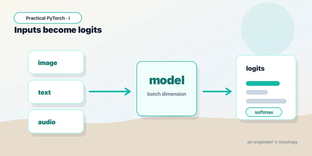
A model doesn’t accept a JPEG, a sentence, or an audio clip. It accepts tensors of a specific shape, scale, and type — and nothing else. The gap between “the thing a human has” (a photo) and “the thing a model eats” (a particular tensor) is bridged by preprocessing, and it’s the part beginners most often get subtly wrong.

For an image classifier, preprocessing usually does three things:

• Resize / crop to the exact dimensions the model was trained on — very often 224×224 pixels. Feed it a different size and you’ll either get an error or quietly worse predictions.
• Convert to a tensor, which also rescales pixel values from the usual 0–255 range down to 0.0–1.0.
• Normalize each color channel by subtracting a mean and dividing by a standard deviation. The model learned on data scaled this way, so it expects to be fed data scaled the same way.

Here’s the single most important thing to internalize: the correct preprocessing is a property of the model, not of you. The mean and standard deviation above aren’t universal constants — they’re the specific numbers this model was trained with. A different model may want different ones. Guessing is how you get a model that runs without error and returns confident nonsense.

The good news is that well-packaged models ship their own preprocessing, so you rarely type those numbers by hand. In torchvision, the weights object hands you a ready-made transform:

from torchvision.models import resnet50, ResNet50_Weights

weights = ResNet50_Weights.DEFAULT      # a specific set of trained numbers
model = resnet50(weights=weights)

preprocess = weights.transforms()       # the exact preprocessing this model wants
tensor = preprocess(img)                # img is a PIL image; tensor is ready to feed
print(tensor.shape)                     # torch.Size([3, 224, 224]) — channels, height, width

Notice we never wrote 224 or any normalization numbers ourselves. We asked the model what it wanted and got back the right pipeline. That’s the pattern to reach for first.

The batch dimension, and why unsqueeze(0)

There’s one more shape gotcha. That tensor is [3, 224, 224] — three color channels, 224 high, 224 wide. But models are built to process many inputs at once for efficiency, so they expect an extra dimension out front telling them how many images are in this call. That leading dimension is the batch dimension.

We have one image, so the batch size is one — but we still have to say so. unsqueeze(0) inserts a new dimension of size 1 at position 0:

batch = tensor.unsqueeze(0)
print(batch.shape)   # torch.Size([1, 224, 224]) → torch.Size([1, 3, 224, 224])

Read it as “a batch of 1 image.” If you forget this step you’ll get a shape-mismatch error that looks scary and means something boring: the model wanted a batch and you handed it a lone image. The fix is almost always one unsqueeze(0).

The output side: the model talks in raw scores

Feed the batch in and the model gives you back numbers — but probably not the numbers you expected:

out = model(batch)
print(out.shape)    # torch.Size([1, 1000])
print(out[0][:5])   # tensor([-1.20,  0.83, -0.41,  2.97, ...])

One thousand numbers (this model knows 1000 ImageNet categories), and they’re all over the place — some negative, none of them looking like a tidy percentage. These raw scores are called logits. A logit is the model’s unnormalized confidence for each class: higher means “more likely,” but the values don’t sum to anything meaningful and you can’t read them as probabilities. Logits are the native language of the output layer; turning them into something human is your job, and it’s two short steps.

Step 1: softmax turns logits into probabilities

Softmax squashes a row of logits into a row of probabilities — every value between 0 and 1, the whole row summing to 1.0. Bigger logits become bigger probabilities, but now they’re on a scale you can actually report to someone:

logits = out
probs = logits.softmax(dim=-1)   # dim=-1 = "across the last axis", i.e. across the 1000 classes
print(probs.sum())               # tensor(1.0000)

The dim=-1 says “normalize along the last dimension.” That last dimension is the row of 1000 class scores, which is exactly what we want softmaxed — not across the batch.

Step 2: argmax for the single best answer

If you just want the model’s top pick, argmax gives you the index of the largest value — the winning class number:

top = probs.argmax(dim=-1)
print(top)                       # tensor([207])  — class index 207

That’s an index, not a name. To turn 207 into “golden retriever,” you look it up in the model’s list of category labels — which, like the preprocessing, ships with the weights:

labels = weights.meta["categories"]
print(labels[top.item()])        # 'golden retriever'

Step 3: topk for the runners-up

A single answer hides useful information. Is the model 99% sure, or torn between two breeds? torch.topk returns the top k probabilities and their indices, so you can show the runners-up:

values, indices = torch.topk(probs, k=5)

for score, idx in zip(values[0], indices[0]):
    print(f"{labels[idx]:<25} {score.item():.1%}")
# golden retriever          88.4%
# Labrador retriever         6.1%
# kuvasz                     1.2%
# ...

Now you’re reading a model the way a human would: a confident top guess, plus a sense of what else it considered. That topk view is often more honest than a lone label.

The two ritual lines, explained

You’ll see two lines wrapped around almost every inference example. They’re not decoration, and now’s a good time to demystify them.

model.eval() switches the model into evaluation mode. Some layers behave differently while training than while running for real — dropout randomly silences neurons during training (a regularization trick), and batch-norm layers update running statistics. eval() turns those training-time behaviors off so the model is deterministic and correct for inference. Forget it and a model with dropout will give you slightly different, slightly worse answers each time. Call it once after loading:

model.eval()

torch.no_grad() tells PyTorch not to track gradients. Remember from Part 1 that autograd is the bookkeeping that lets a model learn — every operation normally records how to compute a gradient later. You’re not training, so that bookkeeping is pure waste: it spends memory and time you don’t need. Wrapping your forward pass in no_grad() skips it, making inference faster and lighter:

with torch.no_grad():
    out = model(batch)

The newer torch.inference_mode() does the same job and is a touch faster still — it’s the modern recommendation, used identically:

with torch.inference_mode():
    out = model(batch)

Either is fine. Use inference_mode() for new code; you’ll see no_grad() everywhere because it’s been around longer.

The general recipe

Here’s the whole thing in one place — and the reason this post matters. This shape is the same for essentially every pretrained model you’ll run, whether it classifies images, transcribes audio, or reads text. The details inside each step change; the four steps don’t.

model.eval()                                # 1. eval mode (do once after loading)

tensor = preprocess(img)                    # 2. preprocess: resize, scale, normalize
batch = tensor.unsqueeze(0)                 #    add the batch dimension

with torch.inference_mode():                # 3. forward pass, no gradient overhead
    logits = model(batch)

probs = logits.softmax(dim=-1)              # 4. postprocess: logits → probabilities
values, indices = torch.topk(probs, k=5)    #    pull out the top answers

Preprocess → batch → forward → postprocess. Internalize those four words and a new model stops being a wall of unfamiliar code. You read its docs for what preprocessing it wants and what its output means, then slot those specifics into a skeleton you already know.

Gotchas

• Wrong preprocessing fails silently. Skip normalization or use the wrong mean/std and the model still runs and still returns a confident answer — just a worse one. No error, no warning. Always use the model’s own bundled transforms when they exist.
• Forgetting the batch dimension. A [3, 224, 224] tensor where the model wanted [1, 3, 224, 224] throws a shape-mismatch error. The fix is almost always a single unsqueeze(0).
• Reading logits as probabilities. Raw output isn’t 0–1 and doesn’t sum to 1. Always softmax before you interpret or display a “confidence.” A logit of 2.97 is not a 297% anything.
• Softmax on the wrong dimension. For a [batch, classes] tensor you want dim=-1 (across classes), not dim=0 (across the batch). Wrong axis gives numbers that sum to 1 in a meaningless direction.
• argmax returns an index, not a label. You still have to look index 207 up in the model’s category list to get “golden retriever.”
• Forgetting eval(). Models with dropout or batch-norm give degraded, non-deterministic results in the default training mode. Call model.eval() once after loading and you’re set.

What’s next

You now understand both ends of a model well enough to run things on your own — which raises a fair question: do you have to write all of this every single time? For a huge range of common tasks, no. The Hugging Face pipeline() wraps preprocess → forward → postprocess into a single call, so you get an answer in two lines and skip the ceremony entirely.

Next: Part 6 — The Fast Path: Hugging Face Pipelines, where one function does everything this post just unpacked — and you’ll appreciate exactly what it’s handling for you.

---

Target keyword(s): pytorch model inputs and outputs, logits vs probabilities, pytorch softmax argmax topk.