From Perceptron to Deep Net: The Famous Little Models You Just Built

Series: Practical PyTorch: Running Models — Foundations — Part 6 of 7

Last post you built a model with your own hands: a single nn.Linear, then a three-layer stack. It probably felt like a warm-up exercise — too small to matter. Here’s the twist: those exact shapes are some of the most famous models in the history of the field. The single layer is a perceptron. The little stack is the network that broke a decade-long deadlock. And the trail from them leads, in a few honest steps, straight to the deep networks you’re about to run.

This post is the short, math-free history that turns your toy into a lineage. Every model below is a handful of lines you can build and print — no training, just recognizing the shapes.

▶ Open the companion notebook in Colab

The perceptron: your single layer, in 1958

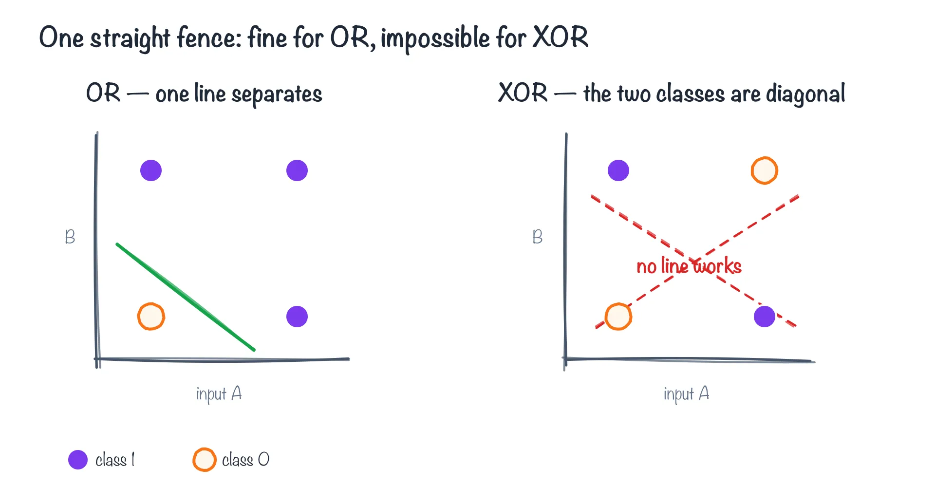
One straight line can fence off OR’s lone corner, but no single line separates XOR’s diagonal classes.

In 1958 Frank Rosenblatt unveiled the perceptron, and within a couple of years had built it into a genuine machine — the Mark I Perceptron of 2560, a room of wires and motor-driven dials that learned to tell simple shapes apart through a camera. Strip away the hardware and the idea is one you now know cold: take some inputs, multiply each by a weight, add them up, and fire a 1 if the total clears a threshold, else a 0. A weighted sum, then a yes/no.

That’s a single nn.Linear with a threshold stuck on the end:

import torch
import torch.nn as nn

perceptron = nn.Linear(2, 1)        # two inputs, one output — Rosenblatt's unit
score = perceptron(torch.tensor([[1.0, 1.0]]))
print(score)                        # a weighted sum; the perceptron fires 1 if it's > 0

If that weighted sum looks familiar, it should: with a single input it’s just y = mx + b — the equation of a line, with the weight as the slope m and the bias as the intercept b. The twist is what the perceptron does with it. It doesn’t read off a y value (that’s what linear regression, in the next section, will do) — it checks which side of the line you land on: w·x + b > 0 fires a 1, everything else a 0. The same line equation, used as a fence between two classes rather than a prediction. That’s also the seed of its famous limitation — a single straight fence can only separate so much.

The perceptron caused a sensation — newspapers wrote about a machine that might one day “walk, talk, see, write.” Then in 1969 Marvin Minsky and Seymour Papert published a book, Perceptrons, with a quietly devastating observation: a single layer like this cannot learn XOR — the simple rule “one or the other, but not both.” No setting of two weights and a threshold can draw the line, because no straight line separates the cases. The result helped cool the early hype: funding and attention drifted away from perceptron-style networks, and the lean years that followed are often called a neural-network “winter.” (Historians still argue over how much the book itself was to blame — plenty else was going on — but the chill was real.)

Hold on to that limitation, because the fix is sitting in your last post.

Linear and logistic regression: one layer, doing real work

Before we fix it, notice that the single layer was never useless — drop the hard threshold and it’s a workhorse you’ve definitely met.

A bare nn.Linear, no activation, is linear regression — the line-of-best-fit from every statistics class:

linreg = nn.Linear(4, 1)            # 4 features in, one number out

Put a sigmoid on the end — a smooth squash into the range 0 to 1 — and you have logistic regression, the most widely used classifier on the planet, the thing predicting spam-or-not and click-or-not in a million production systems:

logreg = nn.Sequential(
    nn.Linear(4, 1),                # weighted sum
    nn.Sigmoid(),                   # squash to a probability between 0 and 1
)
print(logreg(torch.rand(1, 4)))     # e.g. tensor([[0.62]]) — a probability

Swap the sigmoid for a softmax over several outputs and you get softmax regression — which is exactly the single-Linear-plus-softmax classifier you’ll see capping nearly every model in this series. The lesson: one layer, depending on what you tack onto the end, is regression, a probability, or a classifier. It’s a small tool that does a startling amount of real work.

The hidden layer that changed everything

Now the fix. Minsky and Papert were right that one layer can’t do XOR — but stack a second layer between input and output, with a nonlinear ReLU in the middle, and the wall comes down. That extra layer is called a hidden layer, and a network with one is a multi-layer perceptron (MLP). You built one last post:

xor_net = nn.Sequential(
    nn.Linear(2, 2),                # a hidden layer of 2 units
    nn.ReLU(),                      # the nonlinear kink that makes depth count
    nn.Linear(2, 1),
)
print(xor_net)

Once trained (training is the Training Models series — here we just build the shape), this two-layer net solves the very problem that sank the perceptron. And it’s not a one-trick fix. The Universal Approximation Theorem (Cybenko, 1989; Hornik, 1991) proved something remarkable about exactly this shape: a single hidden layer, given enough units, can approximate any continuous function to whatever accuracy you like. One hidden layer is, in principle, enough to represent almost anything.

So why go deeper than one hidden layer? Because “in principle” can demand an absurdly wide layer, while stacking layers builds complexity efficiently — each layer composing on the last. That insight, plus a way to actually train the stacks (backpropagation, popularized in 1986), is the whole ballgame. “Deep learning” is just this: more hidden layers.

The thread so far

Stand back and the lineage is one idea, growing up:

• Perceptron — one weighted sum and a threshold. Couldn’t do XOR.
• Logistic regression — the same one layer with a smooth squash; a probability machine still everywhere in production.
• MLP — add a hidden layer and a nonlinearity; now it can approximate anything, XOR included.

Every step is the previous one plus a little more depth — and every step is built from the exact pieces you assembled by hand last post. The famous models aren’t a different species; they’re your toy, scaled.

But notice what they all share: a Linear layer treats its inputs as a flat, unordered list of numbers. That’s fine for a row of features — and a quiet disaster for an image, where which pixel sits next to which is the whole point. Closing that gap takes a genuinely new kind of layer, and we’ll get there soon.

What’s next

You’ve met the Linear family: the perceptron that started it, the regressions that quietly run the world, and the MLP that broke the XOR deadlock. They’re all nn.Modules made of layers you can name, and not one of them needed math you didn’t have.

You’ve built an MLP — now let’s make one real. In the next post we load trained weights into the exact network you assembled and turn it into a little app that reads handwritten digits. It’s your first capstone, and proof the toy was never a toy.

Next: From Layers to a Live Digit Reader, where the MLP you built becomes something you can actually use.

---

Target keyword(s): perceptron, multi-layer perceptron pytorch, logistic regression pytorch, universal approximation theorem.