What a Model Is Made Of: Build One from a Single Layer Up

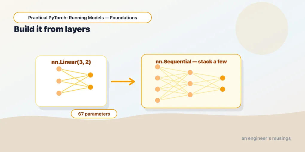
Series: Practical PyTorch: Running Models — Foundations — Part 5 of 7

“A model” is one of those phrases that sounds like it should be mysterious. You download a few hundred megabytes, call it, and answers come out (image labels, sentiments, translations), and somewhere in there is intelligence, supposedly. It’s tempting to treat the whole thing as a sealed box you’re not qualified to open.

So let’s build one — the smallest honest model there is, then a slightly bigger one — with our own hands, out of parts you’ll recognize. Nothing here gets trained; we’re assembling and inspecting, not teaching. By the end the box will be made of glass, because you’ll have made it yourself.

▶ Open the companion notebook in Colab

A model is an nn.Module

In PyTorch, almost every model you’ll ever run is an instance of one base class: nn.Module. That’s the common shape. A language model, an image classifier, a speech recognizer — under the hood they’re all nn.Modules, which means once you can read one, you can read them all.

An nn.Module does two jobs:

• It holds layers, and layers can hold other layers, so a model is really a tree. A big model is a module made of modules made of modules.
• It knows how to do a forward pass: take an input, push it through those layers in order, and produce an output. That’s the thing that happens when you call model(x).

We’ll build up to this gently — the smallest model that exists, then a slightly bigger one we assemble ourselves. (Reading a real, famous model comes over the next couple of posts.) The part we’re not touching is how the numbers inside got to be the right numbers — that’s training, that’s the next phase, and you don’t need it to run anything.

The simplest model: a single nn.Linear

The smallest honest model in PyTorch is one layer. The friendliest one to start with is nn.Linear, which does a weighted sum: it takes some input numbers, multiplies each by a learned weight, adds them up (with a bias), and produces output numbers. Let’s make one that takes 3 numbers in and gives 2 back:

import torch
import torch.nn as nn

layer = nn.Linear(3, 2)   # 3 numbers in, 2 numbers out
print(layer)

Linear(in_features=3, out_features=2, bias=True)

That’s already a complete nn.Module — the very same base class the giant models are built on. Printing it shows its configuration: three inputs, two outputs, a bias. No tree yet, because there’s only one layer.

Inside it live the parameters — the actual numbers, the things training would tune. A Linear keeps two of them, a weight and a bias, and you can look at their shapes:

print(layer.weight.shape)   # torch.Size([2, 3])
print(layer.bias.shape)     # torch.Size([2])

Six weights (one for each input-to-output pairing) and two biases (one per output) — eight numbers in all, and every one is a tensor with a shape, exactly the thing Part 2 made routine. Now push something through it:

features = torch.rand(3)        # the actual input: just 3 numbers, shape [3]
x = features.unsqueeze(0)       # tack on a batch dimension -> shape [1, 3]
out = layer(x)

print(x.shape)                  # torch.Size([1, 3])
print(out.shape)                # torch.Size([1, 2])

Calling layer(x) is a forward pass: numbers go in the top, the weighted sum happens, numbers come out the bottom. That’s the entire job of a model — here on the smallest possible scale.

There’s a small ceremony in that snippet worth pausing on. Your real data is just three numbers — torch.rand(3), shape [3]. But models expect a whole batch of inputs at once (it’s how they stay efficient), even when you have only one. So we unsqueeze(0) — the move from Part 2 — to wrap our lone example in a batch of one, turning shape [3] into [1, 3]. The model reads that leading 1 as “one example in this batch.” You’ll be tacking it on constantly.

Stacking a few: a tiny network

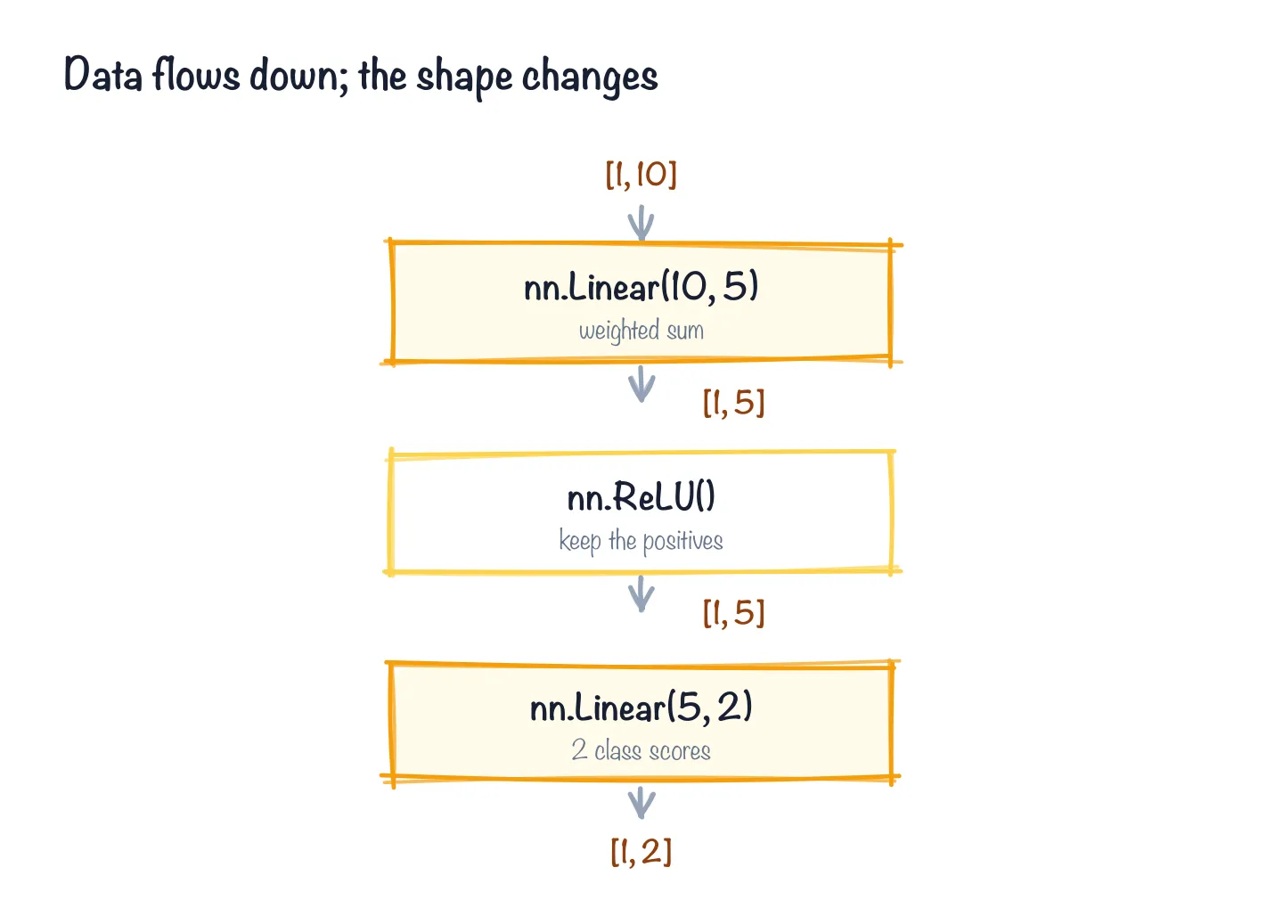
Data flows top to bottom; the shape changes at each layer.

One layer is a model, but real models are layers stacked on layers. nn.Sequential is the simplest way to stack — it just means “run these in order, top to bottom.” Let’s build three layers deep:

net = nn.Sequential(
    nn.Linear(10, 5),   # weighted sum: 10 numbers in, 5 out
    nn.ReLU(),          # keep the positives
    nn.Linear(5, 2),    # weighted sum: 5 numbers in, 2 out
)

print(net)

Sequential(
  (0): Linear(in_features=10, out_features=5, bias=True)
  (1): ReLU()
  (2): Linear(in_features=5, out_features=2, bias=True)
)

That middle nn.ReLU() is the other layer type you’ll meet constantly, and it’s almost comically simple: keep the positives — any negative number becomes zero, positives pass through unchanged. It’s the little nonlinear “kink” between the weighted sums that lets a stack represent complicated relationships instead of collapsing into one big straight line.

That printout is a little tree — three lines, one per layer, each tagged with an index: (0), (1), (2). (Hold on to those numbers; they come back when we name the parameters.) This is a complete nn.Module too: it takes 10 numbers, squeezes them to 5, zeroes out the negatives, then squeezes to 2. Feed it a single example and watch it run — same batch-of-one move as before, now with ten numbers going in:

features = torch.rand(10)       # 10 real input numbers, shape [10]
x = features.unsqueeze(0)       # wrap them in a batch of one -> shape [1, 10]
out = net(x)

print("input shape: ", tuple(x.shape))     # (1, 10)
print("output shape:", tuple(out.shape))   # (1, 2)
print("output:", out)

That call, net(x), is the entire idea of a forward pass, now with more than one stop: data goes in the top, flows down through each layer in turn, and comes out the bottom transformed. The first Linear turns 10 numbers into 5, ReLU clips the negatives, the second Linear turns those into 2. No magic, no training, no math you had to do — just numbers flowing through a stack.

The two output numbers are meaningless here because nobody taught this little net anything; its weights are random. But the mechanics are identical to a real model’s — exactly the mechanics we’ll watch a famous network run, a couple of posts from now.

Counting and naming the parameters

The layers are the structure; the parameters are the actual numbers living inside them. You already peeked at a single Linear’s weight and bias. Across a whole model you can count them all in one line:

total = sum(p.numel() for p in net.parameters())
print(f"{total} parameters")   # 67 parameters

net.parameters() hands you every parameter tensor in the model; .numel() is “number of elements” in one tensor; summing gives the grand total. Sixty-seven numbers — tiny, but counted with the exact same line you’d run on a model with millions. When people say a network “has 100 billion parameters,” this is the count they mean.

To see where those numbers live, walk them by name:

for name, p in net.named_parameters():
    print(name, tuple(p.shape))

0.weight (5, 10)
0.bias (5,)
2.weight (2, 5)
2.bias (2,)

The names are a little map of the model: 0 is the first Linear, 2 is the second — index 1 is the ReLU, which has no numbers of its own, so it never shows up. Every parameter is a tensor with a shape, and that’s genuinely the whole inventory of this model: four tensors, sixty-seven numbers, no secrets. The same named_parameters() walk works on an eleven-million-parameter network; it just prints more lines.

Gotchas

• print(model) shows structure, not the weights. It lists layers and their sizes — it does not dump every number. To touch actual values you go through .parameters() or .named_parameters().
• Random weights ≠ a useful model. Build a fresh nn.Linear or nn.Sequential and its numbers are random, so its outputs are noise. “Pretrained” is what makes a model worth running; those carefully-tuned weights are the whole product. Loading the architecture without the weights gives you an empty shell.
• Inputs need a batch dimension. Our data was ten numbers (shape [10]), but the model wanted them shaped [1, 10] — a batch of one. That’s exactly what the unsqueeze(0) was for. Most models expect a batch even when you have a single input, and forgetting it is the most common shape error you’ll hit. (More on model inputs in the logits and softmax post in the Vision series.)
• Output numbers usually aren’t probabilities yet. A model’s raw outputs (often called logits) are just scores — they can be negative, and they don’t sum to 1. Turning them into “87% confident it’s a cat” is a separate step we’ll cover when we talk about reading outputs.
• for p in model.parameters() will flood a real model’s screen. Our toy has four tensors; a real one has hundreds. Slice it — list(model.named_parameters())[:5] — when you just want a peek.
• You don’t need model.eval() or torch.no_grad() just to look. Those matter when you actually run a pretrained model for real predictions (a few posts out), but building, printing, and counting parameters needs neither.

What’s next

The box is glass now — you built it. A model is an nn.Module: a tree of layers, each holding a pile of numbers, with a forward pass that flows data down through the tree. You made one from a single Linear, stacked a few into a working net, then counted and named every parameter inside. Notice we never trained anything; we only assembled and looked.

Here’s the surprise waiting in the next post: the toy you just built isn’t a toy at all. A single Linear and a small stack of them are the exact shapes of some of the most famous models in the field’s history — the ones that started it.

Next: From Perceptron to Deep Net, where your single layer turns out to be a perceptron, your little stack turns out to have cracked a famous problem, and the trail leads straight to the deep networks you’re about to run.

---

Target keyword(s): pytorch nn.Module, build a neural network pytorch, pytorch nn.Linear nn.Sequential, count model parameters pytorch.