From Layers to a Live Digit Reader
Your first capstone: take the MLP you built by hand, load trained weights into it, and wrap it in a Gradio app that reads handwritten digits you draw — a real, shareable tool, no training required.
Series: Practical PyTorch: Running Models — Foundations — Part 7 of 7
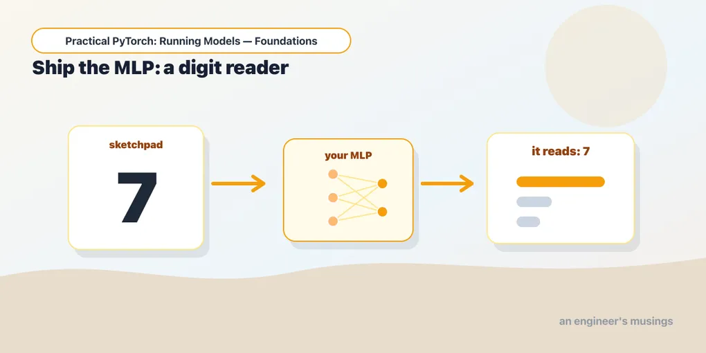
You built an MLP two posts ago — a Flatten, two Linear layers, a ReLU — and it probably still feels like a shape exercise. This post turns it into a thing: an app where you draw a digit with your mouse and the network you assembled tells you what you wrote. Same model, real weights, a web UI, a link you can share. It’s your first capstone.
One honest note up front. A fresh network has random weights and guesses nonsense — the numbers that make it work come from training, which is the Training Models series’ whole job. So we’re not training here; we load weights we trained for you and run them. That’s a completely normal way to use a model (it’s exactly what “pretrained” means), and it lets you ship something real today.
Open the companion notebook in ColabRebuild the exact network
Weights only fit the architecture they were trained on, so step one is to rebuild the MLP from Part 5 — the same layers, the same sizes. A 28×28 digit is 784 numbers in; ten digit classes out.
import torch
import torch.nn as nn

mlp = nn.Sequential(
    nn.Flatten(),                 # 28x28 image -> a row of 784
    nn.Linear(28 * 28, 128),
    nn.ReLU(),
    nn.Linear(128, 10),           # 10 outputs, one per digit
)
Nothing new — you’ve built this exact shape before. Right now it’s full of random numbers.
Load the trained weights
The numbers that make it read digits live in a small file we trained on MNIST (the classic dataset of handwritten digits) and put in the companion repo. PyTorch can pull it straight from a URL and pour it into your model:
url = "https://github.com/book-companion/blog-companion/raw/main/running-models-foundations/weights/mnist_mlp.pt"
state = torch.hub.load_state_dict_from_url(url, map_location="cpu")

mlp.load_state_dict(state)
mlp.eval()
Three things worth naming. load_state_dict_from_url downloads the file once and caches it. A state dict is just a dictionary of the model’s learned tensors, keyed by layer name — load_state_dict copies them into the matching layers, which only works because your architecture matches ours exactly. And mlp.eval() flips the model into evaluation mode (the reflex from Part 5’s cousins): you want it on for inference.
That’s the whole “no training” trick — someone did the learning, saved the numbers, and you loaded them.
Wrap it in a function
A model is just a function: input in, answer out. Our input will be a little drawing; our output, a dictionary of digit scores. The drawing arrives as an image, so the function’s real work is preprocessing it the same way the training data was prepared — grayscale, 28×28, and normalized with MNIST’s mean and standard deviation. Get this wrong and the model returns confident nonsense, so it matters.
from PIL import Image, ImageOps
import torch.nn.functional as F

def read_digit(img):
    if img is None:
        return {}
    img = img.convert("L").resize((28, 28))     # grayscale, 28x28
    img = ImageOps.invert(img)                   # MNIST digits are white on black
    x = torch.tensor([list(img.getdata())], dtype=torch.float32) / 255.0
    x = (x - 0.1307) / 0.3081                    # MNIST's mean and std
    with torch.no_grad():
        probs = F.softmax(mlp(x), dim=1)[0]
    return {str(i): float(probs[i]) for i in range(10)}
It’s the same recipe you’ll see for every model in this series — preprocess, forward, read the output — just small enough to fit on one screen. softmax turns the raw scores into probabilities (the logits and softmax post in the Vision series takes that apart properly); we hand back the ten of them.
Put a face on it with Gradio
Gradio builds a web UI around a Python function — you describe the input and output, it draws the page. We want a little canvas to draw on and a bar chart of the model’s guesses:
import gradio as gr

gr.Interface(
    fn=read_digit,
    inputs=gr.Sketchpad(type="pil", image_mode="L"),
    outputs=gr.Label(num_top_classes=3),
    title="Draw a digit, the MLP reads it",
    description="Scribble a 0–9 and the network you built guesses what it is.",
).launch(share=True)
Run it and a sketchpad appears right in the notebook. Draw a 3, watch the bars jump. share=True gives you a temporary public link (like https://a1b2c3.gradio.live) you can send to someone — they draw, your model reads. The MLP that started life as a shape exercise is now a tool with a URL.
Gotchas
- Preprocessing must match training. The model learned on grayscale 28×28 digits, white-on-black, normalized with a specific mean/std. Feed it anything prepared differently and accuracy collapses with no error message — this is the single most common reason a loaded model “doesn’t work.”
- Architecture must match the weights exactly. Change a layer size and
load_state_dictthrows a shape-mismatch error. The weights and thenn.Sequentialare a matched pair. - The sketchpad’s value shape varies by Gradio version. Newer Gradio may hand
read_digita dict instead of a plain image; if you get an error about.convert, pull the picture out withimg = img["composite"]first. (The code samples here are written against the documented APIs, not run as part of publishing.) - A wobbly drawing fools it. This is a tiny MLP, not a state-of-the-art model — it can mistake a hasty
7for a1. That’s honest: it shows you what a small model can and can’t do, and the Training Models series is where you’d make it better. eval()andno_grad().eval()once after loading;no_grad()around the forward pass. Neither is optional folklore — they’re the inference reflexes from Part 5.
What’s next
You just shipped a model. The MLP you built by hand reads real handwriting and lives behind a link — and you did it by loading weights and wrapping a function, the exact moves the rest of this series leans on.
But your digit reader has a quiet weakness. The moment it Flattens that 28×28 image into a row of 784 numbers, it throws away the fact that pixels have neighbors — and for images, that’s the whole game. Fixing it takes a genuinely new kind of layer.
Next up, the Vision series begins: Teaching a Model to See: Convolution and LeNet, where one new layer fixes everything a Linear gets wrong about images.
Target keyword(s): mlp pytorch app, load state_dict pytorch, gradio mnist, handwritten digit classifier pytorch.
Comments