Twelve Thousand Rows, Fifteen Megabytes

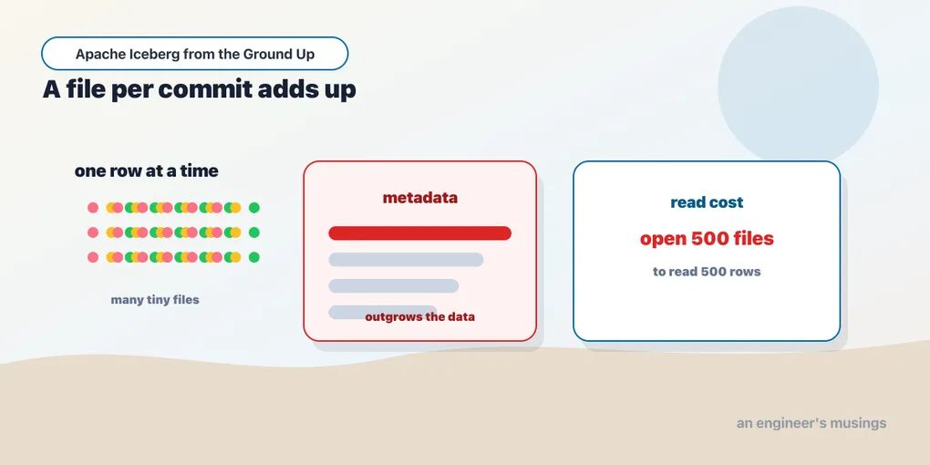
A faster delivery schedule can leave an Iceberg table slower to query, even when the row count barely changes.

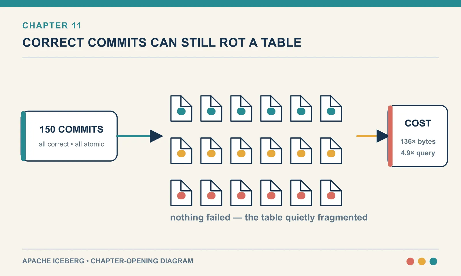
Frequent tiny commits create many small data files and fragmented metadata, increasing storage, planning, and query cost without producing errors.

A team stands up an Iceberg table. It works — queries are fast, the schema evolves without drama, time travel saves somebody’s afternoon once a month. Then the pipeline behind it changes shape. What used to be a nightly batch becomes a micro-batch every minute, because that is what the business asked for and because Iceberg makes it easy. Each batch is one commit. Each commit is atomic. Nobody has to think about it.

Six weeks later the dashboard is slow. Nothing was deleted, nothing was added beyond the usual volume, no query was rewritten. The table has the same number of rows it would have had under the old schedule. It is simply slower — and it is getting worse.

This is the small-files problem, and it is the single most common way an Iceberg deployment goes bad. Understand it precisely, because the folklore is vague — “too many small files, run compaction”. That vagueness leaves you unable to tell whether you have the problem, how badly, or whether the fix worked.

The bookshop orders table lets us separate those questions: write the same rows under different schedules, then compare storage, planning and query cost.

Everything here was run against Apache Iceberg 1.11.0 with PySpark 4.1.3, the iceberg-spark-runtime-4.1_2.13:1.11.0 jar, PyIceberg 0.11.1, and the REST catalog from chapter 5, on Java 21. Every number below came out of that lab.

What the problem actually is

Small files are fine in isolation. They become expensive in a table because reading costs something per file, and that cost does not shrink when the file does. A table can therefore become more expensive to read without gaining any rows.

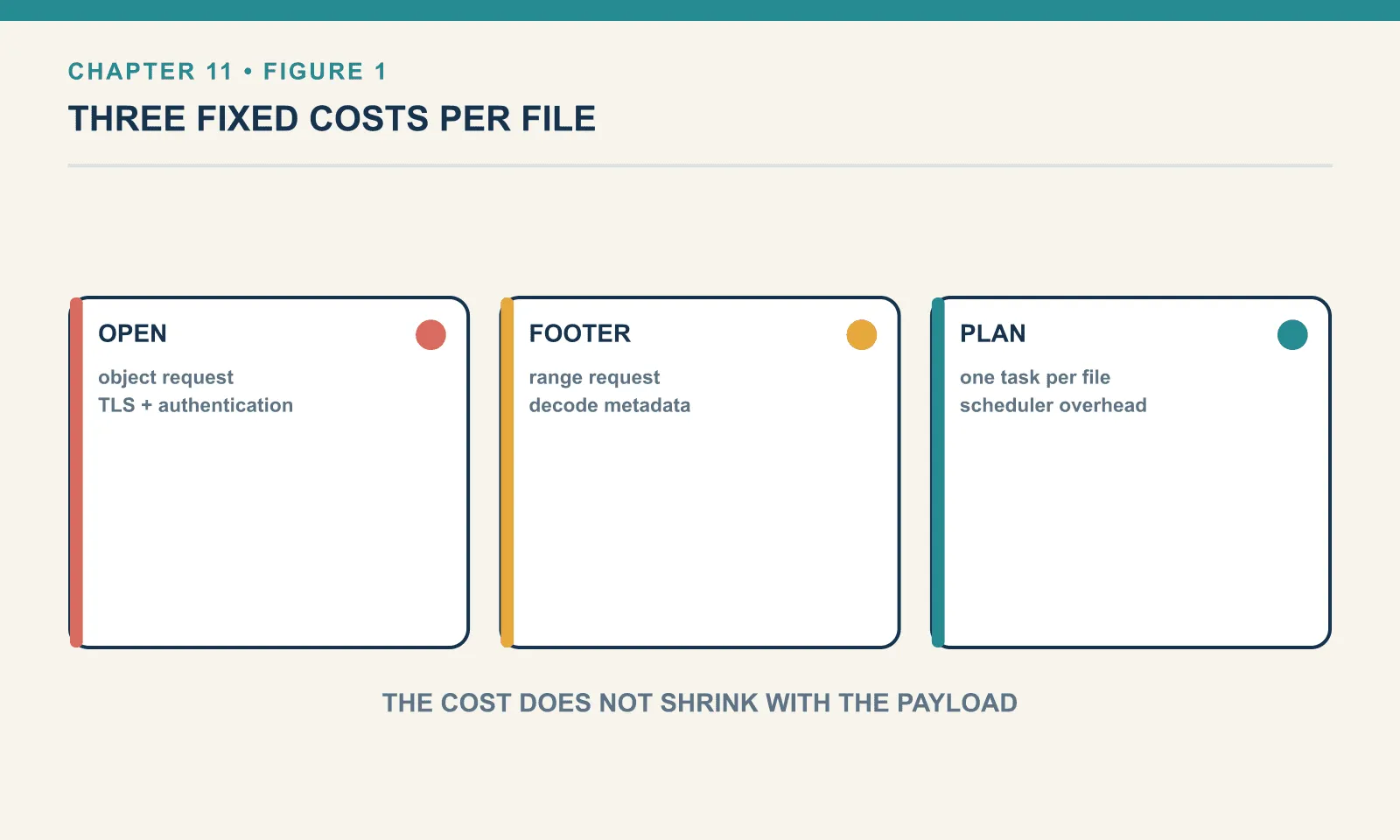
Three separate per-file costs stack up.

Opening the file. Parquet is a footer format. To read anything you fetch the footer, parse the schema and the row-group metadata, then issue reads for the column chunks you want. On a local disk that is a couple of milliseconds. On object storage it is a round trip with a latency floor measured in tens of milliseconds — and it happens whether the file holds ten rows or ten million.

Planning the scan. Before an engine reads a single byte of data it has to decide which files to read. In Iceberg that means walking the manifest list, opening the manifests, and evaluating your filter against each file’s recorded bounds. That work is proportional to the number of entries, not the number of rows behind them.

Losing compression. This one surprises people. Parquet compresses within a row group, and dictionary encoding needs repeated values in the same file to pay for itself. Split the same rows across a hundred files and each file gets its own dictionary, its own header, and a fraction of the repetition. The bytes go up, sometimes dramatically, so you are also reading more data.

None of these depend on the table being big. They depend on the table being fragmented, and the ratio of fragmentation to volume is entirely under the control of how often you commit.

The fixed cost of touching a data file breaks into three parts, and none of them shrinks when the file does: the request that opens the object, the range request that fetches and decodes the Parquet footer, and one planning task per file. Fragmentation multiplies all three by the file count.

Building the wreck

The bookshop orders table, three ways, with identical contents: 12,000 orders spread over ninety days, with order_id, customer_id, book_id, status, amount and order_ts.

The first table is written the way a streaming pipeline writes: 150 separate commits of 80 rows each.

for b in range(150):
    spark.sql(f"""INSERT INTO ice.ch11.orders_stream
                  SELECT order_id, customer_id, book_id, status, amount, order_ts
                  FROM ice.ch11.src WHERE batch_id = {b}""")

The second is the same 12,000 rows in one commit. The third is one commit into a table partitioned by days(order_ts). Here is what each one turned into:

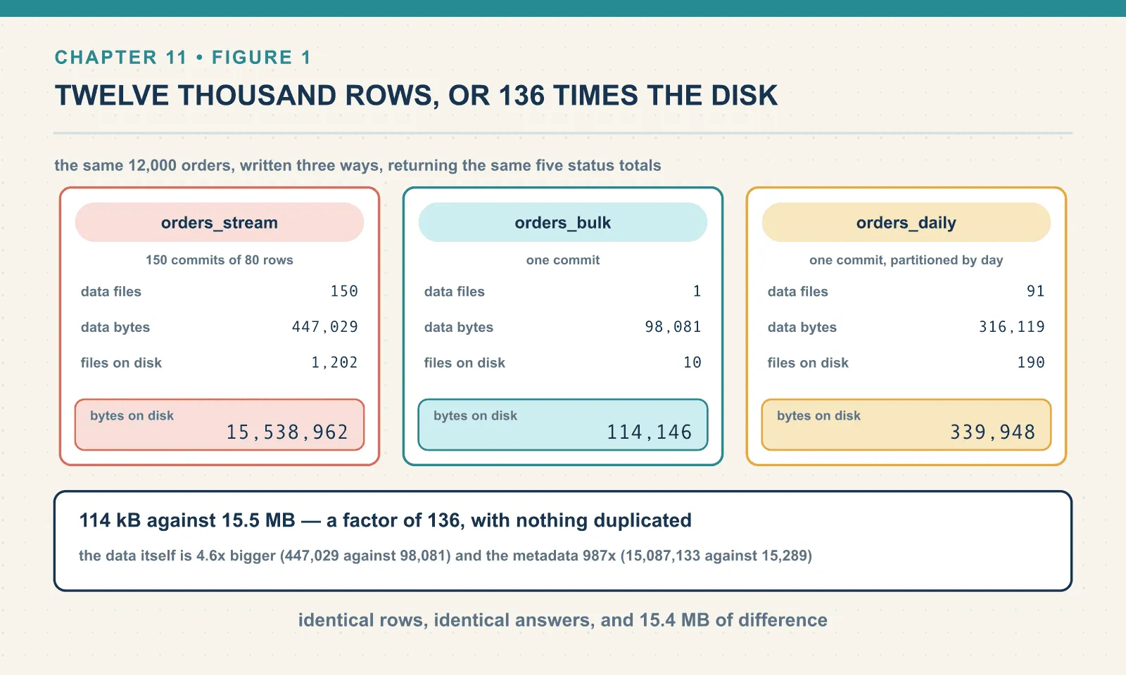
orders_stream  rows=12000 files=150 bytes=447029 avg=2980 min=2871 max=3016
               manifests=51 snapshots=150 metalog=101 disk=1202f/15538962B meta=902f/15087133B
orders_bulk    rows=12000 files=1   bytes=98081  avg=98081 min=98081 max=98081
               manifests=1  snapshots=1   metalog=2   disk=10f/114146B    meta=8f/15289B
orders_daily   rows=12000 files=91  bytes=316119 avg=3473  min=2543  max=3547
               manifests=1  snapshots=1   metalog=2   disk=190f/339948B   meta=8f/20565B

Read the disk column twice. The three tables hold exactly the same 12,000 orders. One of them occupies 114 kB. Another occupies 15.5 MB. That is a factor of 136, and nothing was duplicated — the row counts are identical and both tables return the same answer.

stream agg result: [Row(status='completed', c=2400, s=59988.0), Row(status='paid', c=2400, s=59940.0),
                    Row(status='placed', c=2400, s=59916.0), Row(status='returned', c=2400, s=60012.0),
                    Row(status='shipped', c=2400, s=59964.0)]
bulk   agg result: [Row(status='completed', c=2400, s=59988.0), Row(status='paid', c=2400, s=59940.0),
                    Row(status='placed', c=2400, s=59916.0), Row(status='returned', c=2400, s=60012.0),
                    Row(status='shipped', c=2400, s=59964.0)]

Two of the three costs are already visible in that first block, and they are worth separating.

The data itself got 4.6 times bigger. 447,029 bytes across 150 files against 98,081 bytes in one. Same rows, same columns, same codec. The difference is entirely the compression penalty described above — eighty rows is not enough repetition for dictionary encoding to earn back the per-file overhead. Chapter 1 made the point that Iceberg’s metadata is a rounding error at scale, and it is, but the data bloat here is not metadata at all.

The metadata got 987 times bigger. 15,087,133 bytes against 15,289. Metadata tracks files and snapshots rather than rows, and this table has 150 of each.

Break the metadata directory down by kind and the arithmetic is unremarkable, which is the point:

orders_stream {'crc': 451, 'manifest list (avro)': 150, 'metadata.json': 151, 'manifest (avro)': 150}
orders_bulk   {'crc': 4,   'manifest list (avro)': 1,   'metadata.json': 2,   'manifest (avro)': 1}

One metadata.json, one manifest list and at least one manifest per commit. Nothing pathological happened. The table did exactly what it promised, 150 times.

The directory count and the current snapshot count tell different stories. There are 150 manifests on disk, but the current snapshot references only 51, because Iceberg merges manifests automatically as they accumulate. MANIFEST_MERGE_ENABLED_DEFAULT is true and MANIFEST_MIN_MERGE_COUNT_DEFAULT is 100, both read out of the runtime. And metalog=101, not 151, because the metadata log is capped at 100 previous versions by default: METADATA_PREVIOUS_VERSIONS_MAX_DEFAULT is 100 in the runtime jar. The capped entries did not go anywhere though: all 151 metadata.json files are still sitting on disk, which is a thread chapter 13 picks up and pulls hard.

What it costs to read

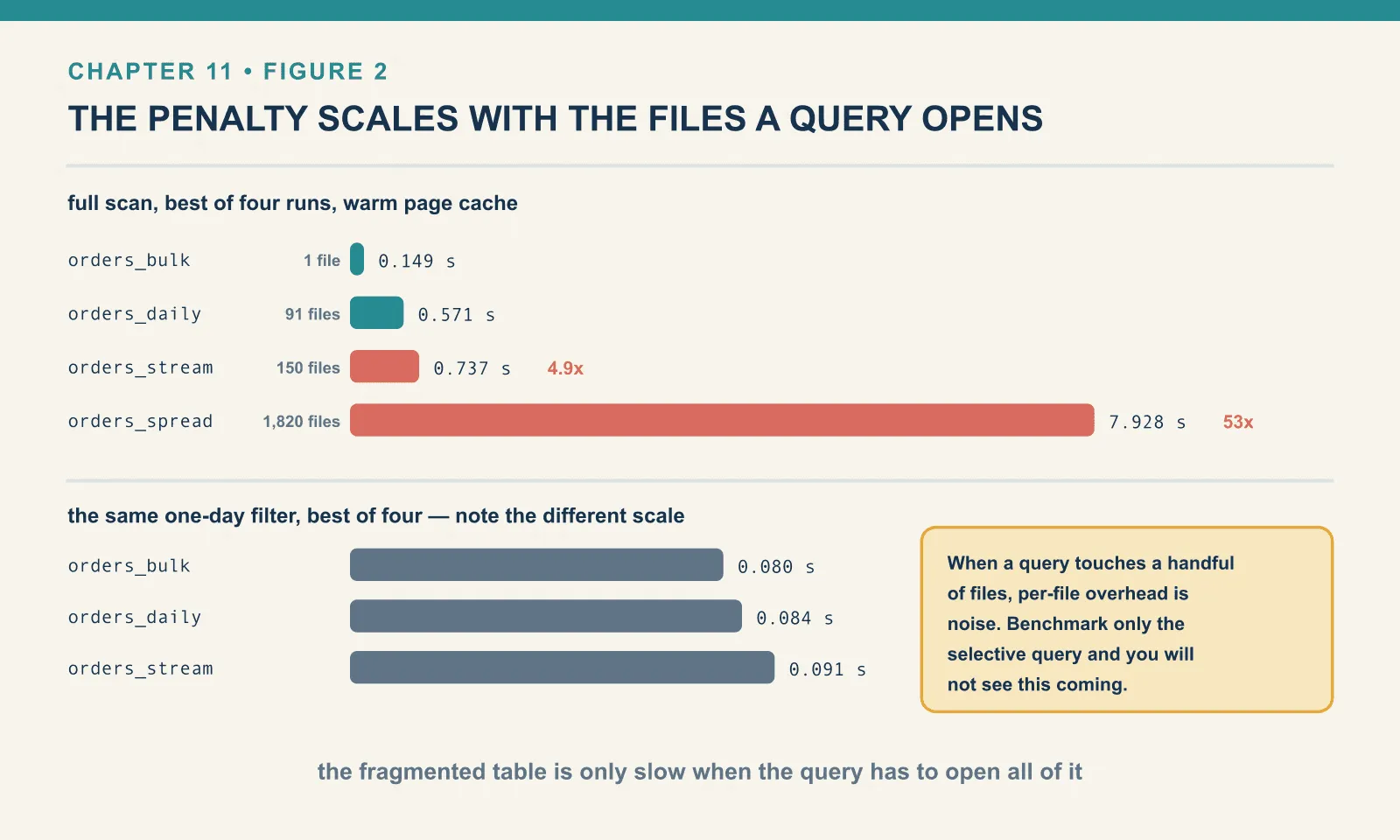
Numbers on disk are only interesting if they show up in a query. Best of four runs, warm:

full-scan agg   orders_stream  runs=['1.351', '0.889', '0.868', '0.737'] best=0.737
full-scan agg   orders_bulk    runs=['0.189', '0.158', '0.149', '0.151'] best=0.149
full-scan agg   orders_daily   runs=['0.626', '0.677', '0.740', '0.571'] best=0.571

one-day filter  orders_stream  runs=['0.141', '0.091', '0.093', '0.091'] best=0.091
one-day filter  orders_bulk    runs=['0.080', '0.127', '0.131', '0.094'] best=0.080
one-day filter  orders_daily   runs=['0.110', '0.090', '0.084', '0.084'] best=0.084

The full scan takes 4.9 times longer on the fragmented table. That is on a laptop, against local files, with the page cache warm and the whole table under half a megabyte. Every one of those conditions flatters the fragmented table. Replace local files with S3 and each of those 150 opens becomes a network round trip.

The one-day filter shows almost nothing, and I am including it because a partial result is more useful than a tidy one. When a query touches a handful of files, per-file overhead is noise. The penalty scales with how many files the query has to open. So a selective query on a well-pruned table can stay fast for a long time while your full scans quietly degrade. If you only benchmark the selective query, you will not see this coming.

A full scan of the same 12,000 rows took 0.149 seconds against one file, 0.571 against 91, 0.737 against 150 and 7.928 against 1,820 — penalties of 4.9 and 53 times. The one-day filter showed almost nothing: 0.080, 0.084 and 0.091 seconds, because it opens only a handful of files either way.

Where the files actually come from

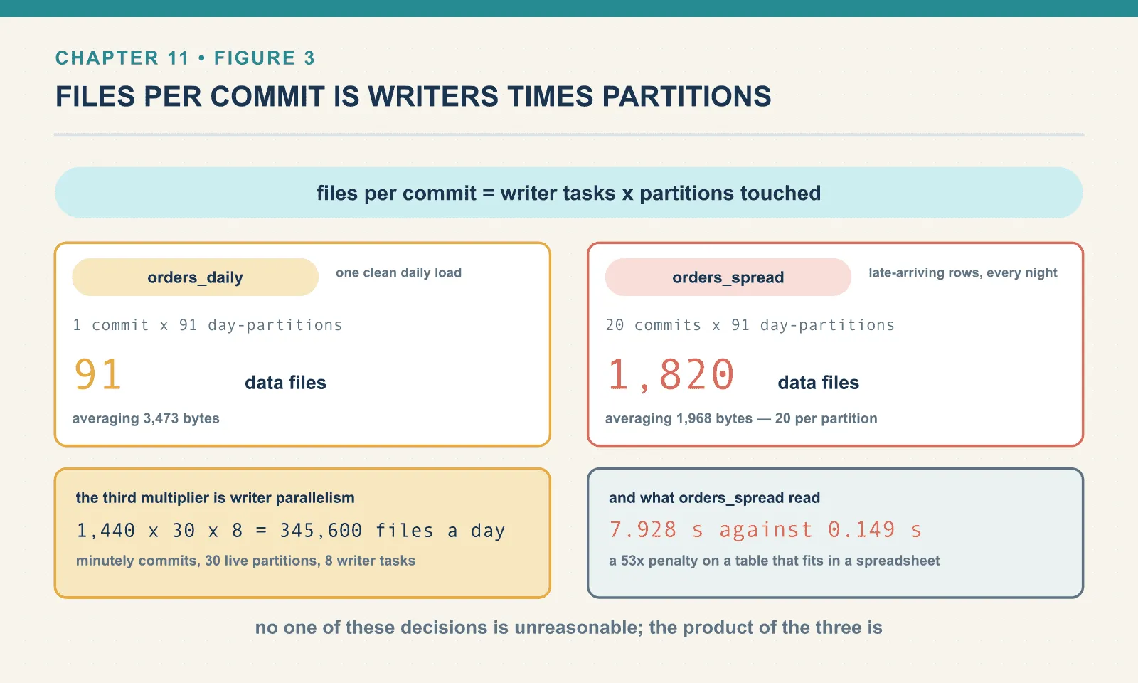
Files per commit is not one. It is writers times partitions, and both multipliers are easy to acquire without noticing.

Look again at orders_daily: one single commit, and it produced 91 data files, one per day-partition, averaging 3,473 bytes. Partitioning a table divides every write by the number of partitions it touches. That is not a flaw — it is the definition of partitioning. But consider two tables partitioned by day. One is loaded daily with that day’s data and produces a single file per commit. The other is loaded daily with late-arriving corrections spanning the history, and produces one file per partition per commit.

The second case is the realistic one, and it is worth seeing at full strength. Twenty nightly loads, each carrying rows scattered across the entire ninety-day history:

partitions: Row(n=91, f=1820, avgf=20)
snapshots: 20
manifests: Row(n=20, b=239926)
disk: 3762 files 4236150 bytes

Twenty commits produced 1,820 data files at an average of 1,968 bytes each. Twenty files per partition, exactly as the multiplication predicts. And the read cost is no longer subtle:

full-scan agg orders_spread: ['9.185', '8.109', '7.931', '7.928'] best 7.928

7.9 seconds against 0.149 for the same 12,000 rows in one file. A 53x penalty, on a table small enough to fit in a spreadsheet.

The third multiplier is writer parallelism. Every task that writes produces at least one file per partition it touches. A job with 200 shuffle partitions writing into 30 date partitions can therefore emit 6,000 files from a single commit. This lab ran on local[2], which is why the numbers above are as gentle as they are.

Put the three together and the arithmetic is unforgiving. A minutely micro-batch is 1,440 commits a day. Give it 30 live partitions and 8 writer tasks, and the ceiling is 345,600 files a day — most of which will be a few kilobytes. Nobody sets out to do that. It is the product of three reasonable-looking decisions, none of which is visibly about file counts.

The other fragmentation, one level up

The files metadata table is not the only thing that fragments. Manifests do too, and they fragment on their own schedule:

orders_stream  manifests=51/387231B
orders_bulk    manifests=1/7420B
orders_daily   manifests=1/12480B
orders_spread  manifests=20/239926B

The stream table carries 387 kB of manifest to describe 447 kB of data. Iceberg’s automatic merging is already working: 150 commits produced 51 manifests rather than 150. But it fires at a threshold and targets 8 MB manifests, so at this scale it barely engages.

This matters because it is a separate condition with a separate fix. Compaction rewrites data files and leaves the manifest tree looking much as it did. A table can have perfectly sized data files and a shredded manifest tree, or the reverse. Chapter 13’s rewrite_manifests is the tool for the second one, and it moves no data at all.

Planning cost, isolated

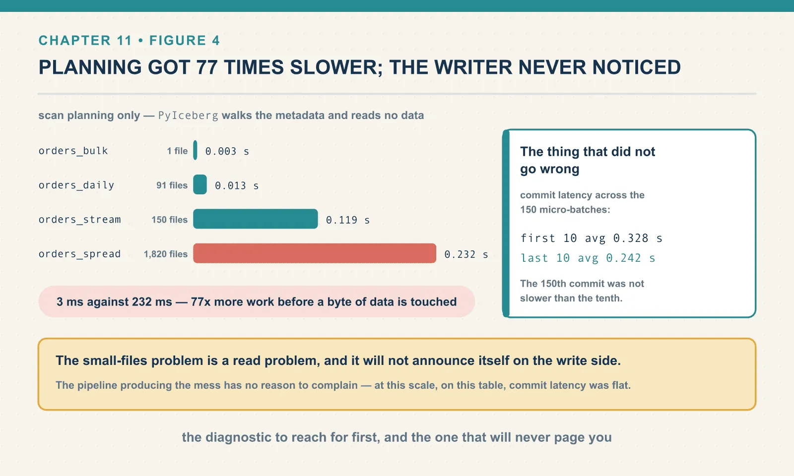
Query time mixes planning and reading together. To see planning on its own, ask PyIceberg to plan the scan and never execute it. This is the microscope role PyIceberg keeps for the rest of the book — no JVM, no data read, just the metadata walk.

t = cat.load_table("ch11.orders_spread")
n = len(list(t.scan().plan_files()))

Best of four, per table:

ch11.orders_stream  files=  150 bytes=  447029 planned=  150 plan_s=['0.122','0.123','0.121','0.119']
ch11.orders_bulk    files=    1 bytes=   98081 planned=    1 plan_s=['0.004','0.004','0.003','0.003']
ch11.orders_spread  files= 1820 bytes= 3581984 planned= 1820 plan_s=['0.249','0.235','0.232','0.244']
ch11.orders_daily   files=   91 bytes=  316119 planned=   91 plan_s=['0.013','0.013','0.013','0.013']

Planning the one-file table takes 3 milliseconds. Planning the 1,820-file table takes 232, which is 77 times more work before any data is touched at all. Planning cost tracks file count almost linearly, and it is paid by every query against the table, including the selective ones that looked fine in the previous section.

This is the measurement I would reach for first when someone says a table “feels slow”. It separates the two halves of the question cleanly. Slow planning is a metadata problem. Fast planning with a slow query is a data-layout problem. They have different fixes, and chapters 12 and 13 handle them separately.

The thing that did not go wrong

Writing stayed fast. Here are the commit times across the 150 micro-batches:

commit seconds: first10 avg 0.328 | last10 avg 0.242

The 150th commit was not slower than the tenth. I expected degradation, because each commit reads the current metadata, writes a new metadata.json containing the whole snapshot log, and swaps the catalog pointer. At 150 snapshots that file is not small.

It did not show up at this scale, and I would rather report that than quietly drop the measurement. Two things are probably holding it back. Automatic manifest merging keeps the manifest count at 51 rather than 150, and the metadata log is capped at 100 entries, so the tracked history stops growing. At thousands of snapshots on object storage this may well look different. What I can say is what I measured, which is that on this table, at this size, commit latency was flat.

That matters practically. The small-files problem is a read problem, and it will not announce itself on the write side. The pipeline producing the mess has no reason to complain.

Planning a scan without executing it took 0.003 seconds against one data file, 0.013 against 91, 0.119 against 150 and 0.232 against 1,820 — 77 times more work before any data is touched. Over the same 150 micro-batch commits, write latency stayed flat: the first ten averaged 0.328 seconds and the last ten 0.242, so the pipeline creating the fragmentation had no reason to complain.

What this lab is not measuring

The local filesystem makes the measured penalties look small. Everything above ran against it. Opening a file cost a page-cache hit and a syscall. On S3, GCS or Azure Blob, opening a file costs an HTTP request — a signed one, with TLS, subject to per-prefix request rate limits and billed per thousand. The Parquet footer read is a separate range request from the column reads — a single small file is at least two requests. The fragmented table above would issue somewhere north of 3,600 requests to answer a full scan that the tidy table answers in a handful.

I did not run that. I have no object-storage numbers in this book, and I am not going to invent a multiplier for them. What I will say is that every mechanism this chapter measured is latency-bound and request-bound, and object storage is worse than local disk on both. Treat the 4.9x and 53x figures as floors.

Why not simply commit less often

Batching more and committing less often can reduce fragmentation — but the table then takes longer to show new orders. Commit frequency is your freshness budget. A table committed every minute is at most a minute stale; a table committed hourly is at most an hour stale. Halving your file count by doubling your batch interval also doubles your worst-case staleness, and for some tables that is a product decision rather than a data-engineering one.

There is also a floor you cannot batch below. A streaming writer with a five-second checkpoint interval commits every five seconds by construction, because that is what gives it exactly-once semantics. You are not going to talk it into ten minutes — the interval is the contract.

Which is why compaction exists. The design that actually works is to let writers commit as often as they need and to fix the layout afterwards, on a schedule, as a separate job. Iceberg’s snapshot model makes that safe — compaction is itself just another commit, readers never see a half-compacted table, and a query running while it happens completes against the file list it started with.

Seeing it coming

Every measurement above came out of metadata tables, which means you can put all of it on a dashboard. There is no need to list a bucket or shell into anything.

The single most useful query is a file-size profile:

SELECT count(*)                                             AS files,
       CAST(avg(file_size_in_bytes) AS INT)                 AS avg_bytes,
       CAST(sum(file_size_in_bytes)/1048576.0 AS DECIMAL(10,3)) AS total_mb,
       CAST(count(*) FILTER (WHERE file_size_in_bytes < 32*1024*1024) * 100.0
            / count(*) AS INT)                              AS pct_small
FROM ice.ch11.orders_stream.files

Run against each of the three tables:

+-------------+-----+---------+--------+---------+
|t            |files|avg_bytes|total_mb|pct_small|
+-------------+-----+---------+--------+---------+
|orders_stream|150  |2980     |0.426   |100      |
|orders_bulk  |1    |98081    |0.094   |100      |
|orders_spread|1820 |1968     |3.416   |100      |
+-------------+-----+---------+--------+---------+

The pct_small column compares against 32 MB. Iceberg’s own default target is much larger: WRITE_TARGET_FILE_SIZE_BYTES_DEFAULT reads 536870912 straight out of the 1.11.0 runtime, which is 512 MB. Thirty-two megabytes is my own threshold for “this file is not paying for the cost of opening it”. It sits an order of magnitude below the target, so the alarm fires on genuine fragmentation rather than on normal variation. Every table here is at 100 percent, including the healthy one, because 12,000 orders is a toy. On a real table this column is the alarm — and it is the one number I would page on.

A size histogram is the next thing to look at, because the average hides bimodal distributions where a healthy table has picked up a tail of tiny files:

+------+-----+-----+------+
|bucket|files|rows |bytes |
+------+-----+-----+------+
|a <8KB|150  |12000|447029|
+------+-----+-----+------+

Then partitions, which tells you whether the fragmentation is spread evenly or concentrated in the partitions your queries actually hit:

SELECT partition, file_count, record_count
FROM ice.ch11.orders_spread.partitions
ORDER BY file_count DESC LIMIT 5

And manifests and metadata_log_entries, which cover the metadata side that files does not see. A table with a healthy file layout can still have a bloated manifest tree, and that is a real condition with its own fix.

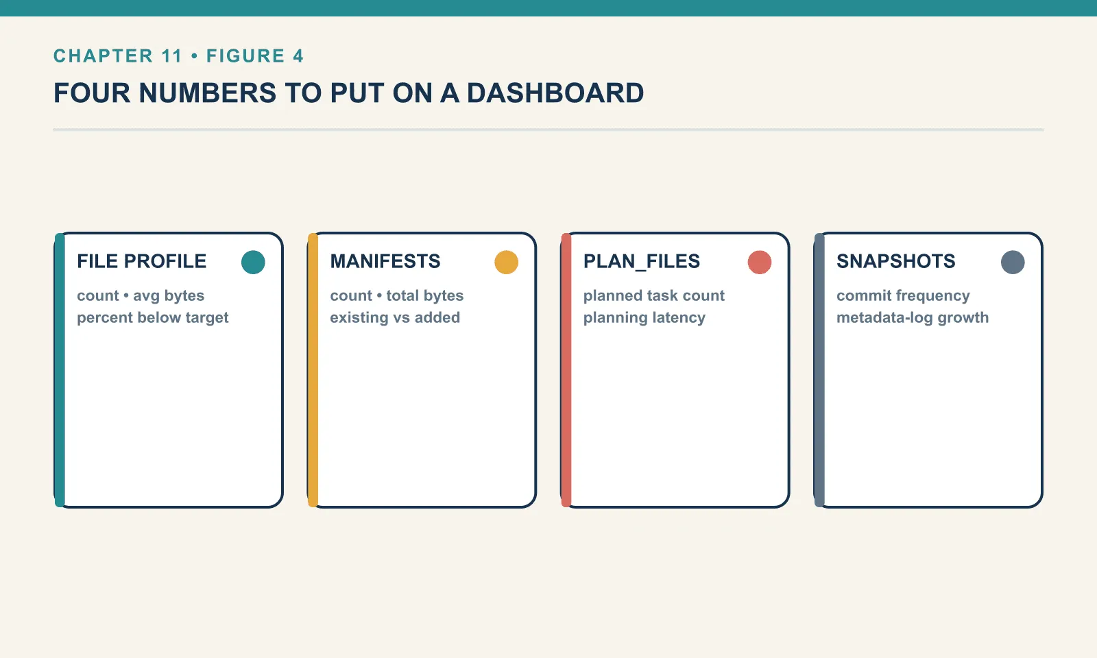
Four numbers are enough for an alert:

file count and average file size, from .files
files per partition, from .partitions, worst partition rather than mean
manifest count, from .manifests
snapshot count, from .snapshots

If you want a single rule: when the average data file in an actively-queried table drops below about 32 MB, or a partition you filter on exceeds a few dozen files, you have work to do.

Four metadata signals worth putting on a dashboard, all of them queryable without listing a bucket: the file profile from the files table, giving count, average bytes and the percent below target; manifest count and total bytes from the manifests table; planned task count and planning latency from plan_files; and commit frequency and metadata-log growth from the snapshots table.

When this is not a problem

The instinct after a chapter like this is to compact everything nightly. Resist it, because compaction is not free. It rewrites data, which costs compute and — on object storage — request charges. It creates a new snapshot, so it makes your table bigger until you expire the old one. And it competes for commits with your writers.

Three cases where the right answer is to leave it alone.

The table is small and fully scanned. If the whole thing fits in memory and every query reads all of it, per-file overhead on a few dozen files is not what is slowing you down.

The table is append-only, written once a day, and already lands one file per partition. It is not fragmenting. Compaction has nothing to do, and as chapter 12 shows, it will politely tell you so and change nothing.

The fragmentation is confined to a hot tail you never scan. A table partitioned by day, where only the last two days are fragmented and every query filters to the last hour, is fine. Compact the tail on a schedule and ignore the history.

The general shape: fragmentation costs you at read time, in proportion to how many fragmented files your queries actually open. If the answer is “not many”, you do not have a problem yet.

Final thoughts

The uncomfortable part of the small-files problem is that nothing goes wrong. No error, no warning, no failed job — every one of those 150 commits was correct, atomic and fast. The table returns exactly the right answer at every point. It just costs 136 times the storage and 4.9 times the query time to do it. And by the time anyone notices, there are six weeks of commits behind the problem rather than one.

The remedy is one procedure call, covered next. The harder decision is where it is needed: which table, which partition, and which queries pay for the fragmentation. The metadata tables already expose the evidence. Tracking file size, files per partition, manifests and snapshots gives you a baseline against which to judge both the damage and the repair.

Set up the four numbers before you need them. The table that is quietly rotting is never the one you are watching.

Next: Compaction