Changing the Shape of a Table That Already Has Data

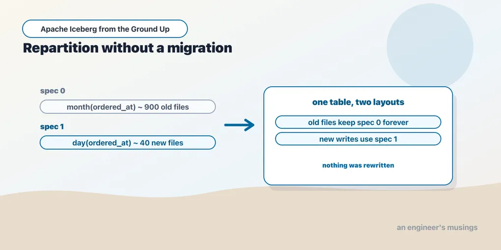
You partitioned the bookshop orders by month. The shop was doing a thousand orders a day, and a month was a sensible amount of data to keep in one place. Two years later it is doing a million a day, every month partition is enormous, and every query that wants one day reads thirty.

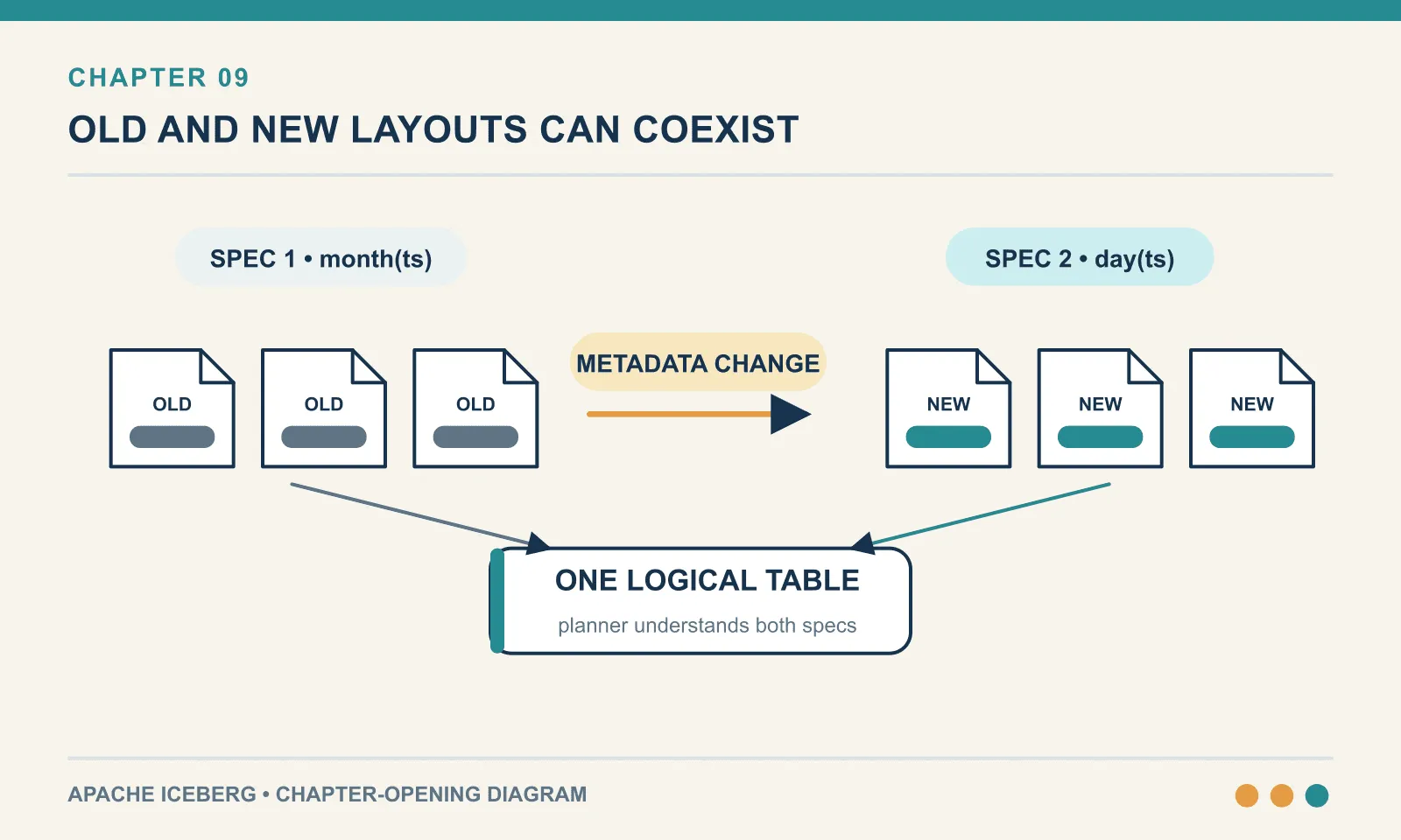
In Hive this is a project. Partitioning is a directory structure, so changing it means writing the entire table again into a new layout. Then checking the copy, swapping the location, and finding out afterwards which downstream job had the old path hard-coded. Teams put it off for years, which is why so many tables in the wild are partitioned for the volume they had when somebody created them.

In Iceberg it is this:

with t.update_spec() as u:
    u.remove_field("ordered_at_month")
    u.add_field("ordered_at", DayTransform(), "ordered_at_day")

That command completed in milliseconds on a table with data in it, moved no bytes, and did not even record a snapshot. New writes can use day partitions immediately. The existing month-sized files remain, so a faster query over the old data still requires work.

Same environment as the rest of this arc: PyIceberg 0.11.1, a SQLite catalog, a local warehouse, no JVM.

The spec is metadata, and files remember theirs

The metadata from chapter 8 already allows more than one partition spec:

"default-spec-id": 0,
"partition-specs": [ { "spec-id": 0, "fields": [ … ] } ]

partition-specs is a list. default-spec-id points at the one new writes use. And every data file’s manifest entry records the spec ID it was written under. Those three facts are the whole feature.

Here is the month-partitioned bookshop, two thousand June orders in a single partition:

spec 0: [ 1000: ordered_at_month: month(8) ]
rows: 2000 files: 1
one-day query under month partitioning: files 1 of 1 rows 200

Evolve it:

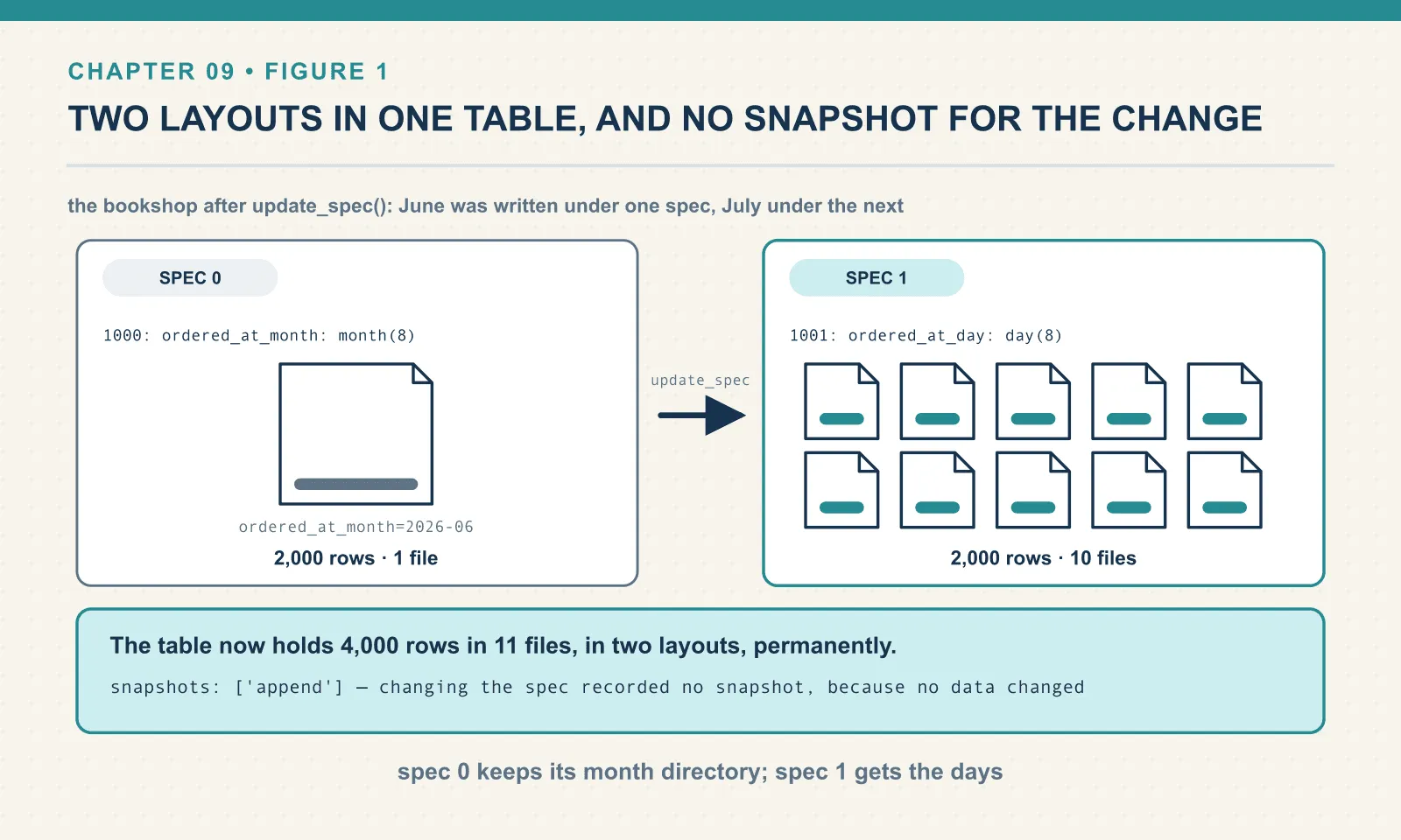
spec now: [ 1001: ordered_at_day: day(8) ]
specs retained: {0: '[1000: ordered_at_month: month(8)]',
                 1: '[1001: ordered_at_day: day(8)]'}
default-spec-id: 1  last-partition-id: 1001

Both specs are kept, the new one is the default, and the new partition field got ID 1001. Partition field IDs come from the same never-reused counter as schema field IDs, for the same reason. An old file’s partition value is recorded against a field ID, and reusing that ID would silently reinterpret it.

Now the important negative result:

rows: 2000 files: 1
dirs: ['ordered_at_month=2026-06']
snapshots: ['append']

One file, still in the month directory, and the snapshot list still has exactly one entry. Changing the partition spec is not a snapshot. No data changed, so there is nothing for a snapshot to describe. It is a metadata-only update — the same shape as the schema changes in chapter 7. A reader that had the table open before the change and refreshes afterwards sees the same rows in the same files, planned slightly differently.

Write July, which goes in under the new spec:

rows: 4000 files: 11
dirs: ['ordered_at_day=2026-07-01', 'ordered_at_day=2026-07-02', …,
       'ordered_at_day=2026-07-10', 'ordered_at_month=2026-06']

Two layouts in one table, side by side, permanently. This is the state Hive could not represent, and the reason repartitioning there was a rewrite. A Hive table has one directory structure, and the metastore assumes it.

What the metadata does with two specs

The partitions metadata table shows the union of every partition field across every spec, with nulls where a field does not apply:

  spec_id= 0 {'ordered_at_month': 677, 'ordered_at_day': None}                    records= 2000 files= 1
  spec_id= 1 {'ordered_at_month': None, 'ordered_at_day': datetime.date(2026,7,1)} records=  200 files= 1
  spec_id= 1 {'ordered_at_month': None, 'ordered_at_day': datetime.date(2026,7,2)} records=  200 files= 1
  …

The nulls distinguish the two layouts. June’s file has no daily partition value because it predates that field; July’s files have no monthly value because their spec does not use it. The listing preserves both without pretending they share one layout.

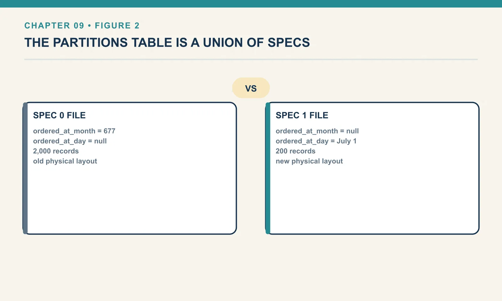
Query planning handles both. Each manifest is planned against the spec its files were written under, and the results are unioned.

The measurement that matters

Changing the spec left June’s file untouched, so the useful comparison is query work on either side of the change. These five filters show the records the planner had to read:

  a June day (old spec)    files=  1 of 11  records_read= 2000  rows_returned= 200
  a July day (new spec)    files=  1 of 11  records_read=  200  rows_returned= 200
  all of July              files= 10 of 11  records_read= 2000  rows_returned=2000
  all of June              files=  1 of 11  records_read= 2000  rows_returned=2000
  spanning the seam        files=  2 of 11  records_read=  400  rows_returned= 400

Line one and line two are the same query against two months of the same table. July reads two hundred records to return two hundred. June reads two thousand to return two hundred — ten times the work. The June data is still in one month-sized file, and the finest thing the old spec can express is a month.

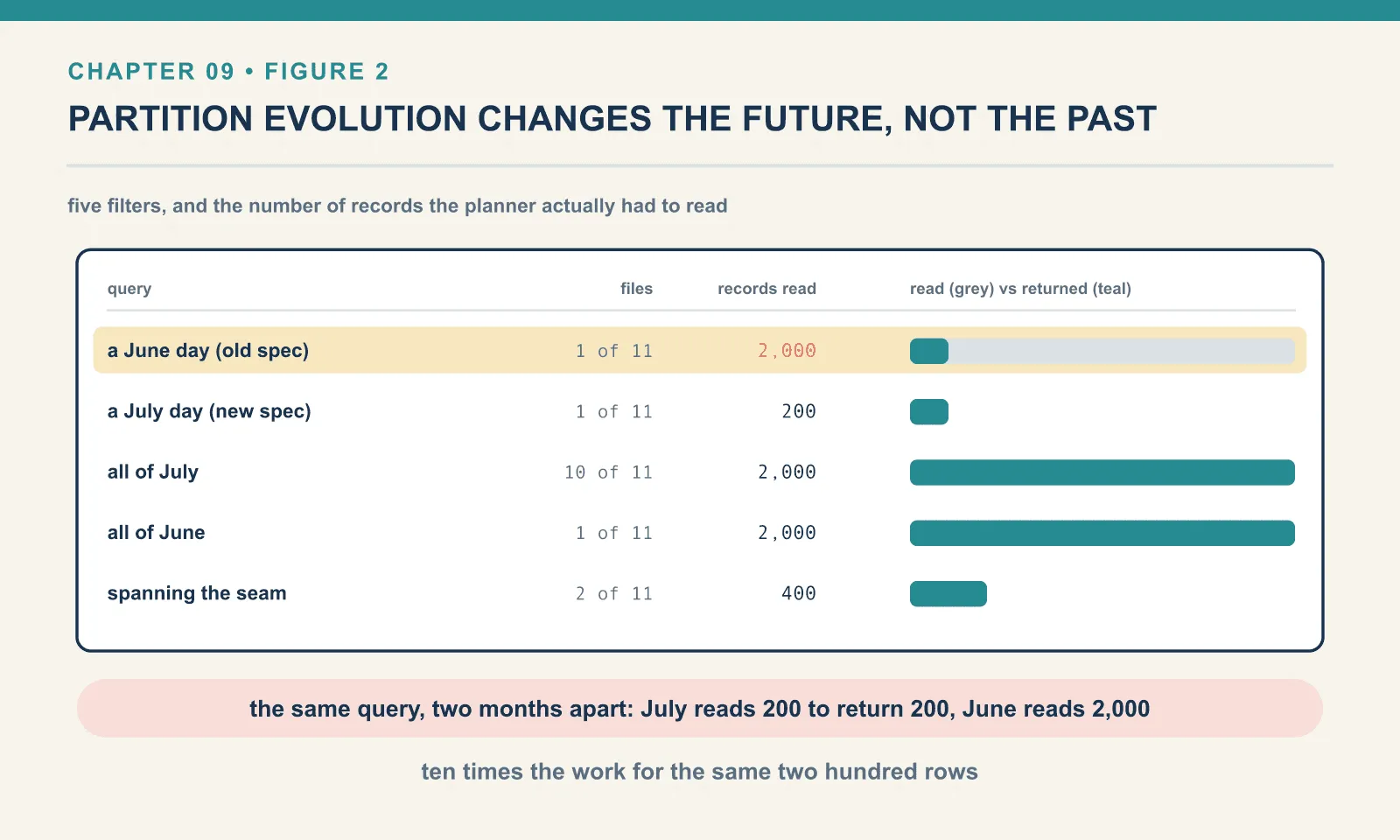
Partition evolution changes the future, not the past. Every file written before the change keeps its old spec and its old pruning granularity forever, or until something rewrites it. The command is free; the benefit accrues only to data written afterwards.

That is the right trade — a metadata change that improves new writes immediately and costs nothing is strictly better than a migration you never schedule. But it has to be understood as what it is. If yesterday’s query pattern is slow because of two years of month partitions, evolving the spec will not fix yesterday. You will need to rewrite those files, and the rewrite runs under the current default spec.

PyIceberg cannot do that rewrite. Its entire maintenance surface is one method:

maintenance surface: ['expire_snapshots']

rewrite_data_files, the Spark procedure in chapter 12, can rewrite those old files. PyIceberg can change the spec and expose its effect on planning, but it cannot perform the maintenance that brings existing data into the new layout.

The rules, found by trying

Field IDs are never reused. Add a field, remove it, add it back:

spec:              [1001: ordered_at_day: day(8), 1002: country: identity(4)]
after removing it: [1001: ordered_at_day: day(8)]
re-added:          [1001: ordered_at_day: day(8), 1003: country2: identity(4)]
last-partition-id: 1003 | specs: 4

Four specs retained after three edits, and the re-added country field is ID 1003, not 1002. Every spec the table has ever had is kept, because files out there reference them by ID.

The spec refers to its source column by ID, so a rename does not touch it. Rename ordered_at to placed_at and the spec still says:

schema: ['order_id', 'customer_id', 'book_title', 'country', 'quantity', 'amount', 'status', 'placed_at', 'channel']
spec still: [1001: ordered_at_day: day(8), 1003: country2: identity(4)]
query by the new name: files 1 rows 200

The partition field is still called ordered_at_day while the column is called placed_at, and pruning works perfectly. day(8) names field 8, and field 8 is the same field it always was. The stale name is cosmetic, and you can rename the partition field too if it bothers you.

You cannot drop a column the spec depends on:

ValidationError: Cannot find source column for partition field: 1001: ordered_at_day: day(8)

Remove the field from the spec first, then drop the column. The order is not negotiable — and the error says why.

You can partition a table that was never partitioned, and un-partition one:

spec: [] files: 1
spec now: [1000: d: day(8)]
one-day query on the OLD files: 1 of 1  records_read 2000
after one append under the new spec: 2 of 11  records_read 2200  rows 400
back to unpartitioned: [] | specs kept: 2

The same lesson in miniature. Partitioning an existing table costs nothing and does nothing for the data already in it. The one-day query still reads all two thousand old records, and after one partitioned append it reads 2,200 to return 400. Going back to unpartitioned reused the existing empty spec rather than creating a third.

And void is how a field gets neutralised rather than removed:

added a void field: [1000: country: identity(4), 1001: country_void: void(4)]

The void transform maps every value to null. It exists because some implementations, and format v1 tables, cannot simply drop a partition field from a spec. They replace it with void instead, which keeps the field position while making it carry no information. If you see a void field in a spec in the wild, you are looking at the scar from a removal.

Sort orders: the other lever

Partitioning is a hard, physical guarantee with a hard, physical cost — chapter 8 measured it as one file per partition per commit. There is a second lever, under-used, that gives you a softer guarantee for no file-count cost at all.

Recall the mechanism from chapter 8. Every manifest holds per-column lower and upper bounds for every data file, and the planner skips files whose bounds exclude your predicate. Those bounds are only as useful as the data’s ordering. A file whose customer_id runs from 1000 to 1249 excludes nothing. A file whose customer_id runs from 1062 to 1093 excludes almost everything.

Sorting the data before you write it turns the bounds from noise into an index. And Iceberg lets you declare the ordering on the table:

with ts.update_sort_order() as u:
    u.asc("customer_id", IdentityTransform())
    u.desc("ordered_at", IdentityTransform())

default sort order: []
after update: [ 2 ASC NULLS LAST
                8 DESC NULLS LAST ]
default-sort-order-id: 1

"sort-orders": [
  {"order-id": 0, "fields": []},
  {"order-id": 1, "fields": [
     {"source-id": 2, "transform": "identity", "direction": "asc",  "null-order": "nulls-last"},
     {"source-id": 8, "transform": "identity", "direction": "desc", "null-order": "nulls-last"}]}]

Source IDs again, a version history again, and a null-order because nulls have to go somewhere. Sort fields can take transforms too, so bucket or truncate orderings are expressible.

The declaration is not enforced

Now append unsorted data to that table and look at what actually landed:

file rows: 2000
customer_id bounds: 1000 - 1249
first 12 customer_ids as stored: [1007, 1014, 1021, 1028, 1035, 1042, 1049, 1056, 1063, 1070, 1077, 1084]
is the file actually sorted by customer_id? False
sort_order_id recorded on the data file: None

The table says its sort order is ascending by customer_id. The file PyIceberg just wrote is not sorted by customer_id, and its manifest entry does not even claim to be. sort_order_id is null.

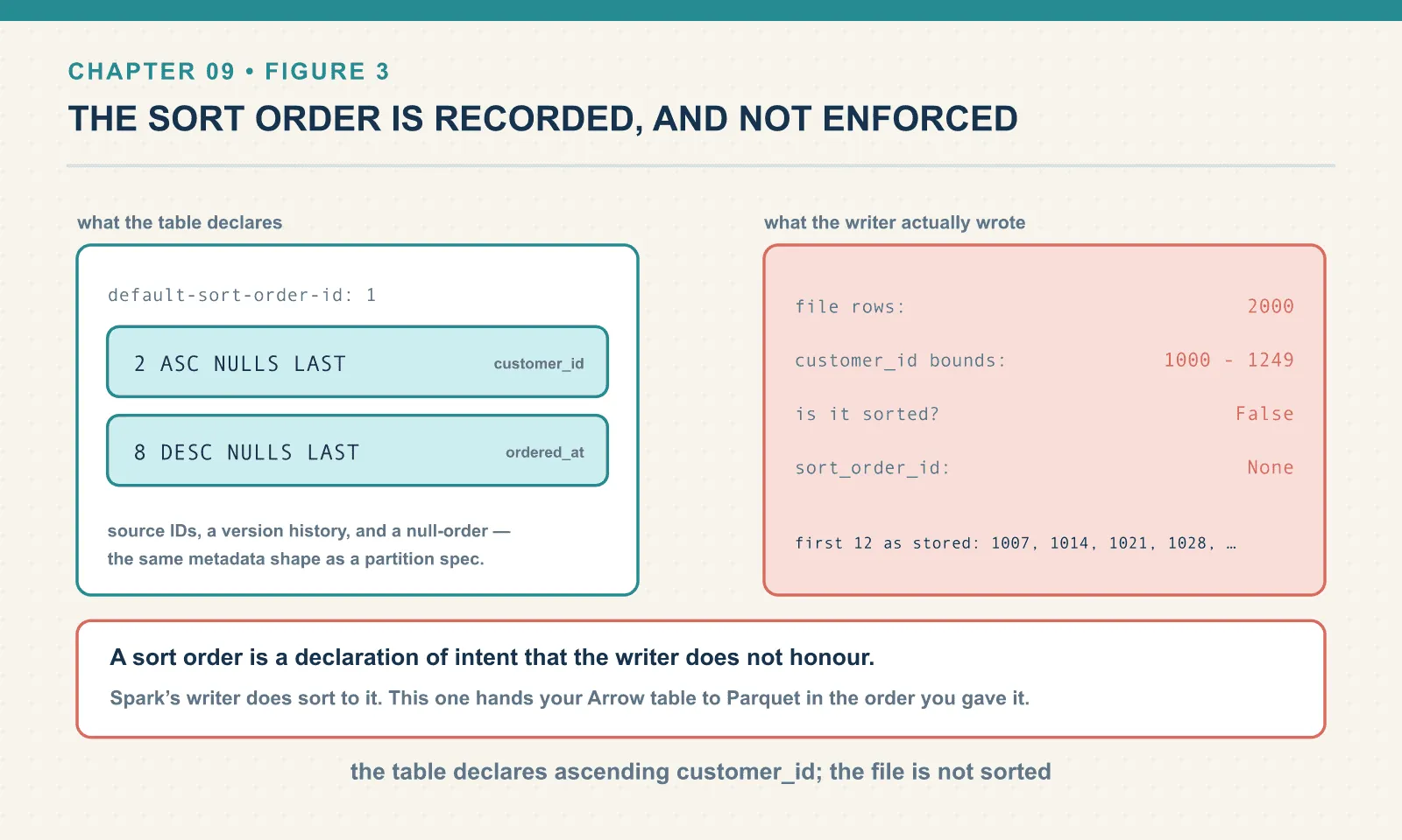
In PyIceberg 0.11.1 a sort order is a declaration of intent that the writer does not honour. It is metadata telling other engines what this table wants. It is not a constraint on the write path. Spark’s Iceberg writer does sort to the table’s declared order. PyIceberg hands your Arrow table to Parquet in the order you gave it.

Reading documentation will not tell you this, because from the documentation’s point of view nothing is wrong. The sort order is a table property, and honouring it is a writer’s choice. From your point of view it is very wrong. Set a sort order in PyIceberg, assume your files are sorted, and every query you tuned on that assumption is running on unsorted data.

What sorting is worth, measured

So sort it yourself. Eight thousand rows, written as eight files of a thousand, twice: once in arrival order, once sorted by customer_id first.

srt = big.sort_by([("customer_id", "ascending")])

unsorted files: 8   presorted files: 8
  unsorted   customer_id bounds per file: [(1000, 1249), (1000, 1249), (1000, 1249), (1000, 1249)] …
  presorted  customer_id bounds per file: [(1000, 1031), (1031, 1062), (1062, 1093), (1093, 1124)] …

The row count, file count and bytes are identical. Only the grouping of rows changed, and the bounds now describe a slice of the key range in each file. That gives the planner a reason to skip files.

  customer_id = 1077 on unsorted   files 8 of 8   rows 32
  customer_id = 1077 on presorted  files 1 of 8   rows 32
  range on unsorted   files 8 of 8  rows 640
  range on presorted  files 1 of 8  rows 640

Same answers, an eighth of the I/O, from a sort_by call before the write. No partitions were created, no extra files exist, and there is no per-commit cost the way partitioning has.

Sorting has to be global, and the first key is the design

Two ways to get that wrong, both common, both measurable.

The first is sorting each batch as you write it. That is what a distributed writer does naturally: every task sorts its own partition of the data and writes a file. Same eight thousand rows, same eight files, each one internally sorted:

locally sorted    bounds [(1000, 1249), (1000, 1249), (1000, 1249)] … files scanned 8 of 8
globally sorted   bounds [(1000, 1031), (1031, 1062), (1062, 1093)] … files scanned 1 of 8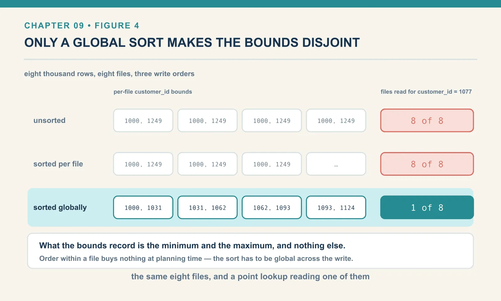

Locally sorted files are perfectly sorted inside and completely useless outside. Every file still spans the whole key range, so every file’s bounds still match every predicate. What the bounds record is the minimum and the maximum, and nothing else. Order within a file buys you nothing at planning time. The sort has to be global across the write for the ranges to become disjoint.

The second is choosing the sort key by importance rather than by selectivity. Sort by country then customer_id:

country-then-customer: customer lookup files 7 of 8   rows 32
country-then-customer: country  lookup files 2 of 8   rows 1600
customer-sorted      : country  lookup files 8 of 8   rows 1600

A sort helps its prefix and degrades sharply after it. Leading with a five-value column pins the customer lookup back to seven files of eight, because within a country the customer ids still span everything. Leading with customer_id gives a perfect customer lookup and no help at all on country.

No ordering is good for both. That is the honest limitation of a linear sort, and the reason multi-dimensional clustering exists. Choose the column your most expensive query filters on, and accept that the second column is nearly free only if it correlates with the first.

The measurements explain why partitioning and sorting need different operating habits:

• Partitioning is a guarantee. It survives any write order, it lets the planner eliminate files without reading any statistics, and it costs at least one file per partition per commit.
• Sorting is an optimisation. It costs nothing structurally and it makes column bounds selective on as many columns as your sort has prefixes. It is also only as good as the discipline of whatever wrote last.

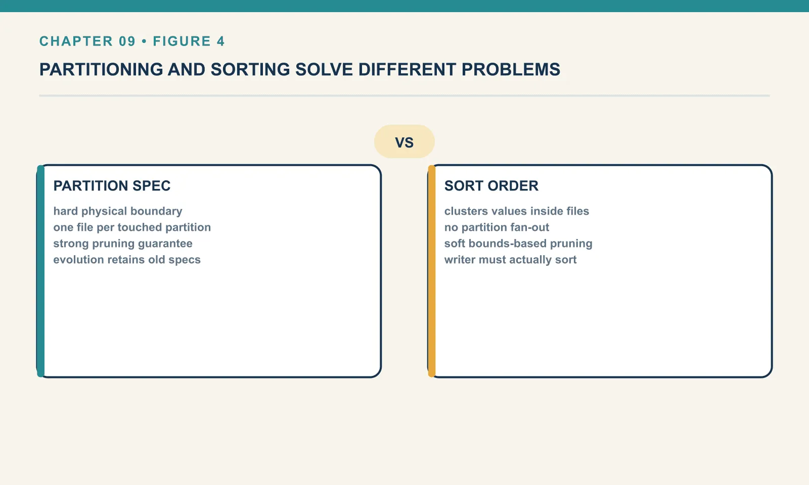
Which is why they compose rather than compete. Partition by the coarse dimension everything filters on; sort within the partition by the next thing people filter on:

files: 12 partitions: 10
one day: 2 files of 12, rows 800
one day + one customer: 2 files, rows 3

At this scale the second filter bought nothing, and I am showing it rather than hiding it. With only two files in the day, there was nothing left to prune. Sorting pays when a partition holds many files, which is the situation any table worth partitioning is in. Do not expect to see the benefit on two thousand rows.

There is a multi-column version of this: ordering data so that filters on several independent columns all prune well, usually via a Z-order or Hilbert curve. It is real, it is useful, and it is a rewrite strategy in Spark’s rewrite_data_files. Chapter 12. I have not run it here.

When not to reach for either

Do not evolve a spec casually. Every spec is retained forever, planning has to consider all of them, and the partitions table becomes progressively harder to read. Two or three specs over a table’s life is a table that adapted. Nine is a table nobody understood.

Do not evolve a spec expecting a speed-up on old data. The measurement above is the whole point: 2,000 records read to return 200, indefinitely. If old data matters, budget the rewrite at the same time as the spec change. The rewrite is the expensive half.

Do not set a sort order you are not going to maintain. An unmaintained sort order is worse than none. It is a claim in the metadata that somebody will eventually believe, and in PyIceberg specifically it is a claim nothing enforces.

And do not sort on a column nobody filters on. The pruning benefit comes from comparing predicates with column bounds. A convenient sort key earns nothing here if the queries never use it.

Final thoughts

The pattern across this whole arc is one idea repeating. A table is a list of files plus a description of how to interpret them. Changing the description is cheap; changing the files is expensive. Iceberg’s job is to let you change the description without pretending you have changed the files.

Snapshots did it for the file list. Field IDs did it for the schema. Partition specs and sort orders do it for the layout, and the honest accounting is the same each time. The metadata operation is instant, and the data written under the old regime stays as it was until something rewrites it. What you gain is that the rewrite becomes optional, incremental, and schedulable — instead of a migration standing between you and a decision you have already made.

Four chapters in, everything has been additive. Rows arrive and rows accumulate. The only way we have removed one is to rewrite a whole file without it. Chapter 6 measured that: three hundred and sixty records deleted and two hundred and eighty-eight rewritten, to remove twenty.

That arithmetic gets worse in exactly the way you would expect at scale. It is the reason for the next chapter, which is also where this book stops being able to do everything in Python.

Next: Deleting a Row From an Immutable File