The Partition Column That Isn't There
In Hive the query had to know the layout. Here the table knows it. This chapter runs the query that prunes ten files to one without naming a partition anywhere, then measures what happens when you pick the wrong transform.
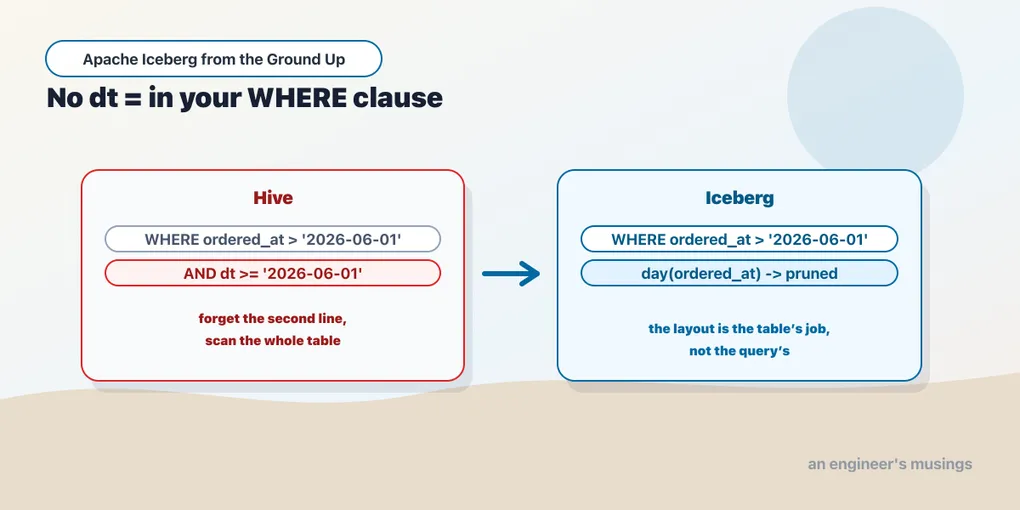
A query can return the right answer while reading years of orders to find one day. Hive’s partitioning left the query author responsible for avoiding that waste, as chapter 1 described:
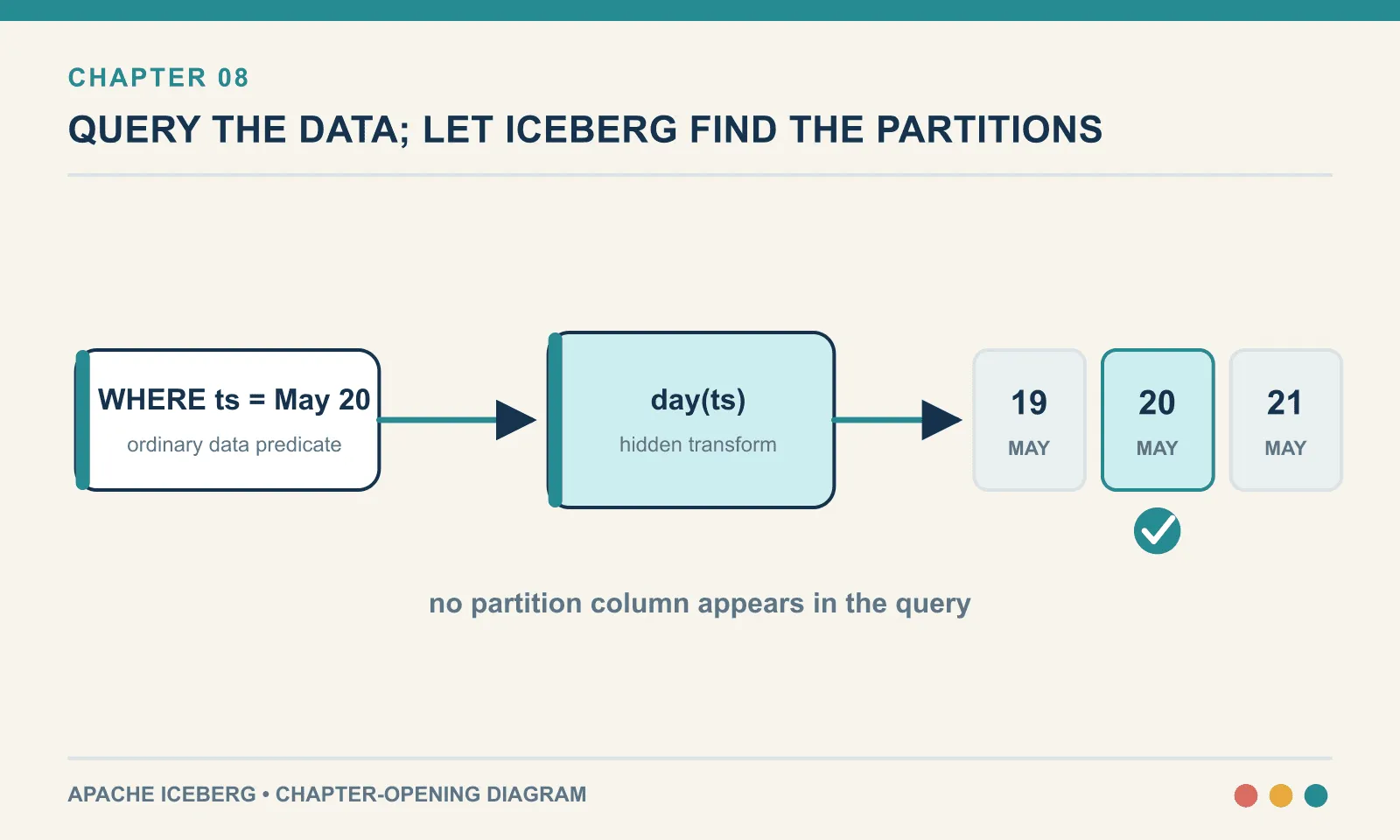
Partitions were physical, and the query had to know. If a table was laid out by
dt=2026-05-20/, then filtering on an actual timestamp column would not prune anything. You had to filter on the partition column, by name, in the shape the layout expected. Get it wrong and you scanned the whole table while the query still returned correct results, so the only symptom was cost.
Correct results make this failure hard to catch. The dashboard returns the right number and nobody is paged; the unnecessary scan appears only as cost. A query for one day can quietly read four years of orders.
The fix Iceberg applies is small and slightly startling: the partition column stops being a column. You do not write it, you do not query it, and it is not in the schema. The table records the function that produces it, and the query planner applies that function to your predicates on your behalf.
Everything here runs on PyIceberg 0.11.1 against a SQLite catalog and a local directory. The bookshop orders table now has the shape chapter 7 left it in — order_id, customer_id, book_title, country, quantity, amount, status, ordered_at, channel — and two thousand orders spread over ten days of June.
The declaration
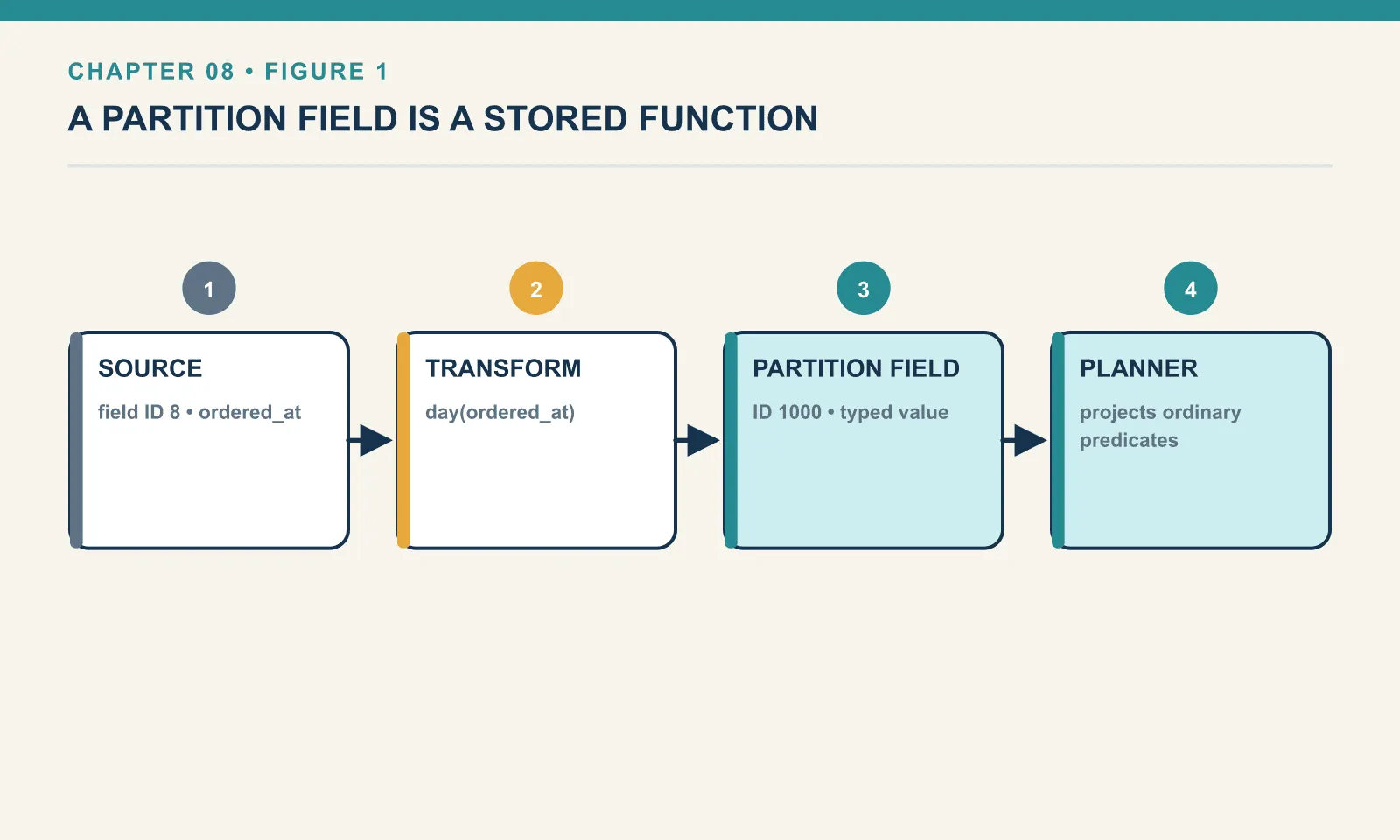
A partition spec is a list of (source column, transform, name):
from pyiceberg.partitioning import PartitionSpec, PartitionField
from pyiceberg.transforms import DayTransform

spec = PartitionSpec(
    PartitionField(source_id=8, field_id=1000,
                   transform=DayTransform(), name="ordered_at_day"))

t = cat.create_table("bookshop.orders", schema=SCHEMA, partition_spec=spec)
source_id=8 is ordered_at’s field ID from chapter 7. The spec refers to the column by ID rather than by name, so renaming the column does not break the partitioning. field_id=1000 is the partition field’s own ID, from a separate counter that starts at 1000 to keep it clearly distinct from schema field IDs.
Ten appends later, one per day, the warehouse looks familiar:
rows: 2000 files: 10
data dir (first few of 10):
    ordered_at_day=2026-06-01/00000-0-273936d7-….parquet
    ordered_at_day=2026-06-02/00000-0-2d8bc05e-….parquet
    ordered_at_day=2026-06-03/00000-0-e8ee3626-….parquet
    ...
That looks exactly like a Hive table. Say it immediately, then: the directory names are decoration. Iceberg writes them because humans and support engineers benefit from a browsable warehouse, but nothing reads them. The partition value that matters is stored in the manifest, next to the file path, and we will look at it in a moment. Rename every directory and the table would still work; delete the manifests and no amount of correct directory naming would save you.
The query
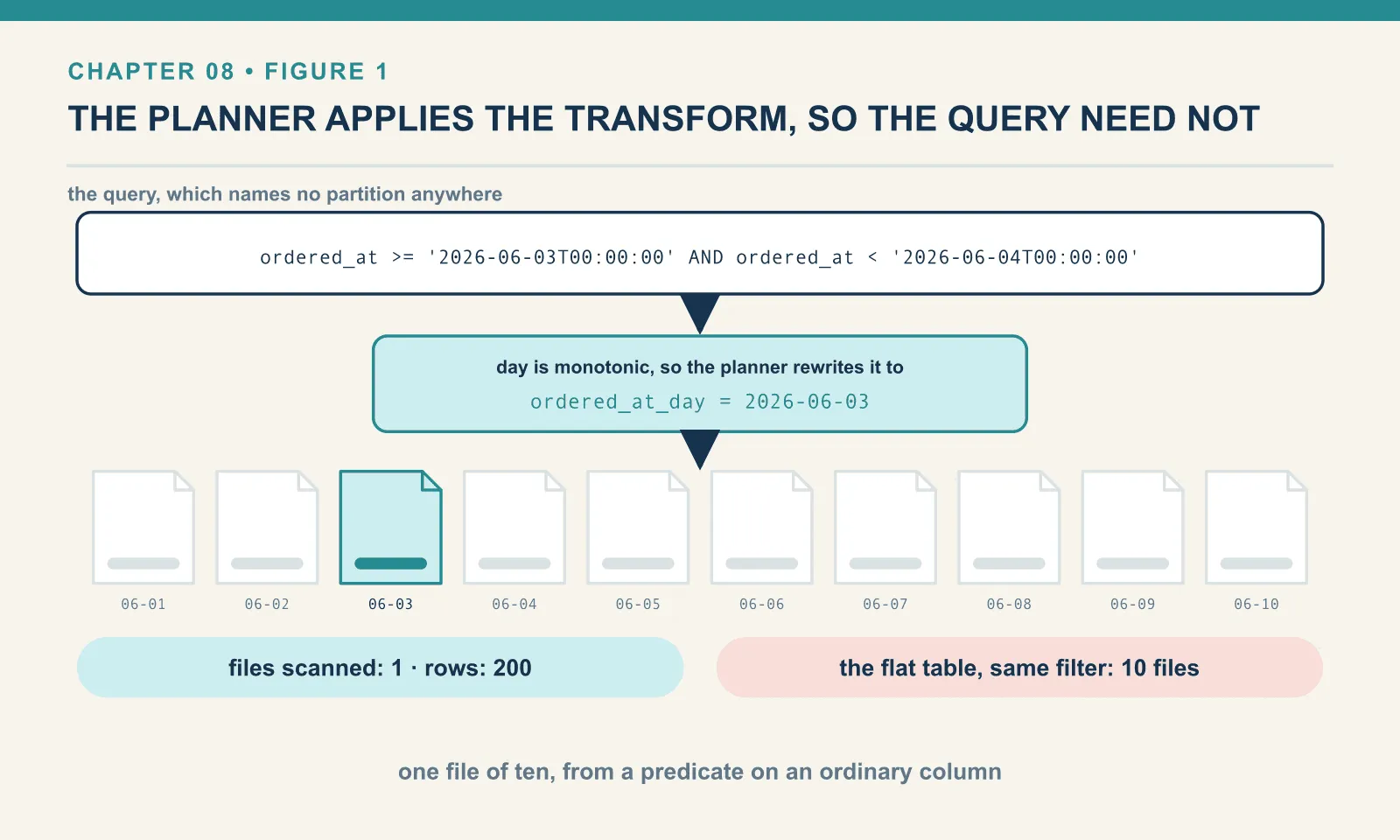
The query asks for one day using only ordered_at. Its file plan shows whether the table can derive the partition constraint:
q = And(GreaterThanOrEqual("ordered_at", "2026-06-03T00:00:00"),
        LessThan("ordered_at",           "2026-06-04T00:00:00"))

len(list(t.scan(row_filter=q).plan_files()))
files scanned: 1 rows: 200
flat table, same filter: files scanned: 10No dt. No partition name. No knowledge of the layout anywhere in the query. The predicate names ordered_at, which is a real column holding a real timestamp, and the planner opened one file out of ten.
What happened is one substitution. The table knows partition values are day(ordered_at). The predicate says ordered_at >= 2026-06-03 AND ordered_at < 2026-06-04. day is monotonic, so the planner rewrites that into a constraint on the partition value, ordered_at_day = 2026-06-03, and drops every manifest entry that fails it. The rewrite happens in the planner, on metadata, before a single Parquet file is opened.
The comparison line in that output is the unpartitioned version of the same two thousand rows. It scanned all ten files to find the same two hundred rows.
The honest part: partitioning is not the only thing pruning
If you build that comparison casually you will get a result that flatters Iceberg for the wrong reason. My first attempt loaded the flat table one day per append, and the one-day query scanned one file out of ten there too. Nothing was partitioned. The pruning was real.
The reason: every Iceberg manifest stores per-column minimum and maximum values for every data file, and the planner uses them.
bookshop.orders_flat_clustered  file0 ordered_at lower=2026-06-10 00:00:00 upper=2026-06-10 23:59:00
bookshop.orders_flat            file0 ordered_at lower=2026-06-01 00:00:00 upper=2026-06-10 23:23:00
bookshop.orders                 file0 ordered_at lower=2026-06-10 00:00:00 upper=2026-06-10 23:59:00
A file whose ordered_at runs from the 10th to the 10th cannot contain a row from the 3rd. It is skipped, partitioned or not. The flat table that pruned had accidentally been clustered by day, because each append happened to hold one day.
The version in the comparison above interleaves all ten days into every file. Its bounds run 06-01 to 06-10, no file can be excluded, and pruning collapses to zero.
Iceberg prunes on both partition values and column bounds. Partitioning guarantees a physical layout regardless of arrival order; statistics describe the layout the writer produced. Already-ordered data can therefore prune well without partitioning — the observation behind chapter 9’s sort orders. Partitioning keeps the guarantee when arrival order changes.
Predicate shapes
The rewrite is not magic and it has a shape. Five filters against the same day-partitioned table:
  day equality window    files=  1  rows=200
  three-day range        files=  3  rows=600
  open-ended >=          files=  3  rows=600
  sub-day window         files=  1  rows= 16
  no time predicate      files= 10  rows=400
A three-day range keeps three partitions. An open-ended >= on the 8th keeps the 8th, 9th and 10th. A two-hour window inside one day still costs a whole day’s file, because the partition granularity is a day and nothing finer can be expressed. And a filter on country alone prunes nothing on the time dimension. That is correct, and it is why the choice of partition column is a query-shape decision rather than a data-shape one.
The column that does not exist
Try to use the partition field the way you would use a Hive partition column:
t.scan(row_filter=EqualTo("ordered_at_day", "2026-06-03"))ValueError: Could not find field with name ordered_at_day, case_sensitive=TrueThere is no such column. It is not in the schema, it is not in the data files, and no query can select it. ordered_at_day is a name for a partition field, a label on a metadata concept. The only place it appears in a reader’s world is inspect.partitions().
For a team migrating from Hive, the adjustment is in the query: filter on ordered_at, the real column. The planner derives the constraint on ordered_at_day; the query cannot address that partition field directly.
Where the partition value actually lives
t.inspect.partitions().to_pylist(){'ordered_at_day': datetime.date(2026, 6, 10)} record_count= 200 file_count= 1
{'ordered_at_day': datetime.date(2026, 6, 9)} record_count= 200 file_count= 1
{'ordered_at_day': datetime.date(2026, 6, 8)} record_count= 200 file_count= 1And per file, in the manifest entry itself:
manifest entry partition value: {'ordered_at_day': datetime.date(2026, 6, 10)}
file path: ordered_at_day=2026-06-10/00000-0-d3690b19-….parquet
The partition value is a typed field stored beside the file path, not a string parsed out of it. That is why there is no MSCK REPAIR TABLE in this book. Nothing is discovered by listing, so nothing can drift out of sync with a listing. A file that is not in a manifest is not in the table, whatever directory it is sitting in.
If that still sounds like a distinction without a difference, set one table property and look at the warehouse:
t = cat.create_table("bookshop.objstore", schema=SCHEMA, partition_spec=spec,
                     properties={"write.object-storage.enabled": "true"})
0000/0010/0001/00100101/ordered_at_day=2026-06-01/00000-0-c04e732f-….parquet
1100/0110/1001/11000011/ordered_at_day=2026-06-02/00000-0-217e1457-….parquet
1101/1000/1110/00110011/ordered_at_day=2026-06-03/00000-0-d27772f4-….parquet
one-day query: 1 of 3 files, rows 200The partition directory now sits underneath a binary hash prefix, so files that would have been adjacent are scattered across the key space. This exists because S3 historically throttled on shared key prefixes, and a table whose hot partition is one prefix is a table with one hot shard. Pruning is unaffected — one file of three, same as before — because the planner was never reading the path.
Pruning happens twice
One more detail from the metadata, because it explains why this scales. Manifests carry summaries too:
t.inspect.manifests().to_pylist()b9f54a08-944b-43aa-a added_files= 1 partition_summaries=
[{'contains_null': False, 'contains_nan': False,
'lower_bound': '2026-06-10', 'upper_bound': '2026-06-10'}]Every manifest records the range of partition values of the files it lists. So planning is two levels: skip whole manifests whose partition range cannot match, then skip individual files inside the ones that survive. On a table with millions of files, a one-day query never opens most of the metadata either. That is the difference between this and a Hive table that had to list storage before it could start.
The spec itself is four lines of the metadata JSON:
"default-spec-id": 0,
"partition-specs": [
  { "spec-id": 0,
    "fields": [ { "source-id": 8, "field-id": 1000,
                  "transform": "day", "name": "ordered_at_day" } ] } ],
"last-partition-id": 1000
Note partition-specs is a list and default-spec-id selects one of them. A table can have several specs at once and files written under different ones. That is chapter 9.
The transforms, measured
There are seven transforms. Here they are, all applied to the same two thousand interleaved rows, one table each:
  hour       partitions=240  files=240  avg_bytes=3713   min=3644  max=3793
  day        partitions=10   files=10   avg_bytes=5532   min=5506  max=5615
  month      partitions=1    files=1    avg_bytes=16420
  year       partitions=1    files=1    avg_bytes=16420
  bucket16   partitions=16   files=16   avg_bytes=5111   min=4721  max=5459
  identity   partitions=6    files=6    avg_bytes=6029   min=4074  max=6443
void partitions=1 files=1 avg_bytes=16420year, month, day, hour extract a time bucket from a date or timestamp. They are not interchangeable with each other at different granularities in one spec — you pick one, and picking is most of the skill.
bucket[N] hashes the value and takes it modulo N. It is for columns with no useful ordering and high cardinality, where what you want is an even spread and the ability to answer point lookups.
truncate[W] cuts a value down: for a string, the first W characters; for a number, rounding down to a multiple of W.
identity uses the value itself. It is the only transform Hive had.
void always produces null. It exists so a partition field can be neutralised without being removed from a spec. That matters when a table has files written under an older spec — chapter 9’s subject.
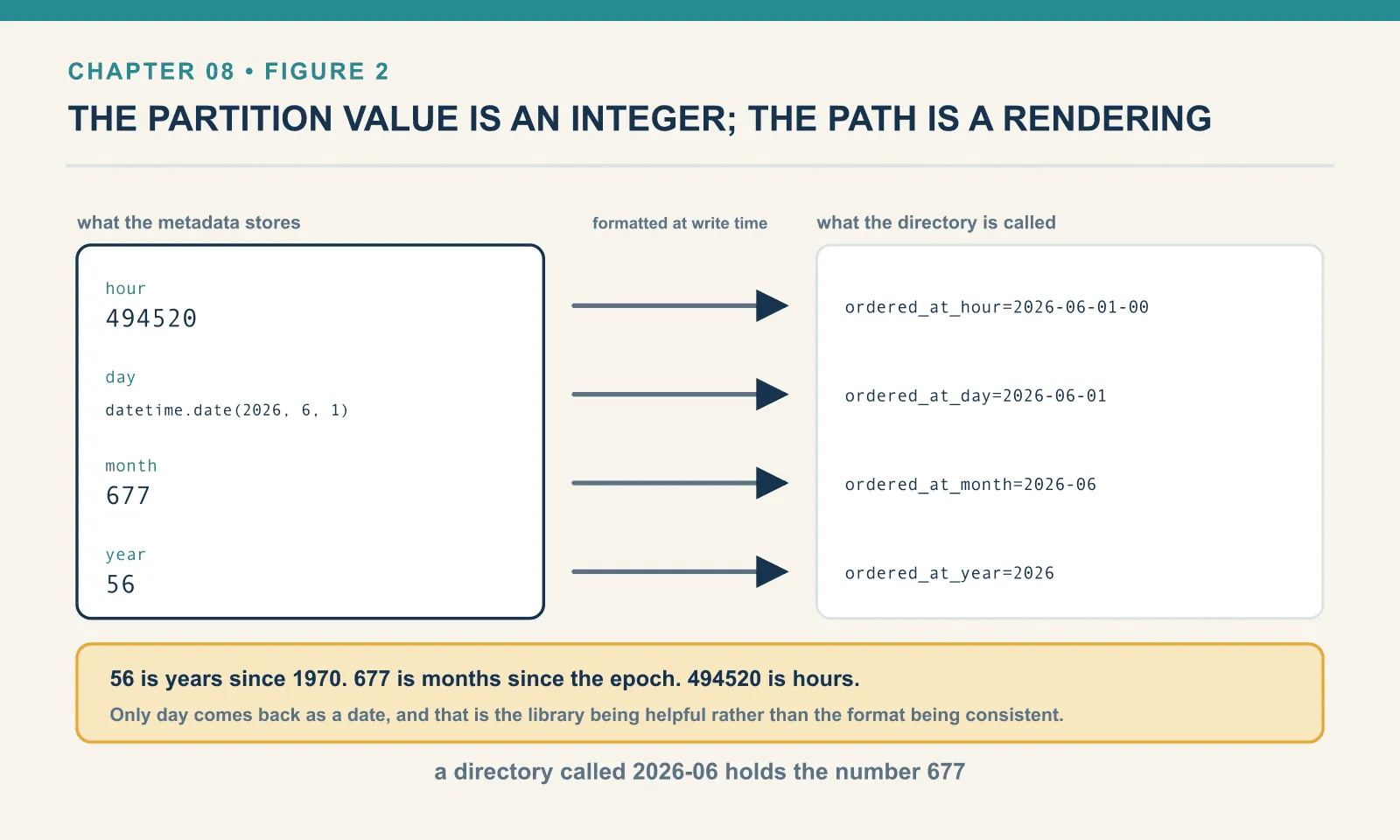
The stored value is an integer, and the directory name is a lie
Print the partition values as PyIceberg reports them and something jumps out:
  hour    sample=[{'ordered_at_hour': 494520}, {'ordered_at_hour': 494521}, ...]
  day     sample=[{'ordered_at_day': datetime.date(2026, 6, 1)}, ...]
  month   sample=[{'ordered_at_month': 677}]
  year    sample=[{'ordered_at_year': 56}]
Hours since the epoch. Months since the epoch. Years since 1970 — 56 is 2026. Only day comes back as a date, and that is PyIceberg being helpful rather than the format being consistent.
Meanwhile on disk:
ordered_at_month=2026-06
ordered_at_year=2026
ordered_at_hour=2026-06-01-00
Human-readable, and produced by formatting the integer at write time. If you ever find yourself parsing partition values, take them from the metadata and know that 677 is a month.
Bucket pruning, and what it cannot do
customer_id = 1007:            files scanned 1 of 16, rows 8
IN(3 ids):                     files scanned 3, rows 24
range on a bucketed column:    files scanned 9 of 16, rows 40
A point lookup on a bucketed column touches exactly one file out of sixteen. That is the reason to bucket at all: a customer-history query on a hundred-million-row table reads a sixteenth of it, with no ordering guarantee required. IN with three values touches three.
The third line is the limitation. A range over a bucketed column cannot use the partition at all, because hashing destroys order — adjacent ids land in unrelated buckets. Nine of sixteen files were still skipped, and that was the column-bounds pruning from earlier doing the work, not the partitioning. Bucket for equality; never bucket a column you filter with > and <.
Truncate, and the collision you should expect
book_title = 'Dune': files 1 of 7, rows 250
truncate partitions: ['Circ', 'Dune', 'Klar', 'Norm', 'Pira', 'Proj', 'The ']
Eight distinct titles produced seven partitions, because truncate[4] maps both The Silent Patient and The Overstory to The . That is not a defect. The transform is allowed to be lossy, and pruning to a partition that contains extra rows is still correct, because the engine applies your real predicate to the rows it reads. Truncation trades precision for a smaller number of partitions, and on real-world strings the prefixes are rarely uniform. Pick the width by looking at your data, not by picking a round number.
Nulls get a partition
ti.append(orders_with_null_country)partitions now: [... {'country_ident': None}]
dirs: ['country_ident=DE', 'country_ident=FR', 'country_ident=GB',
'country_ident=IN', 'country_ident=US', 'country_ident=null']
null query rows: 20
null query files: 1 of 6Nulls are a partition value like any other, the directory is called null, and country IS NULL prunes to that one file. Anyone arriving from Hive will remember __HIVE_DEFAULT_PARTITION__ and the queries that had to know about it. It is gone.
The write side, and where the small files come from
Partitioning changes the shape of every write, and this is the cost people do not budget for. Three appends of three hundred rows each, spread across five days:
  after append 1 -> files: 5   partitions: 5
  after append 2 -> files: 10  partitions: 5
  after append 3 -> files: 15  partitions: 5
An append writes at least one file per partition it touches. Five partitions, three appends, fifteen files, none of them large. A partitioned table cannot merge a new row into an existing file, because data files are immutable. So every commit that spans N partitions adds at least N files.
Now scale that thought. A pipeline running hourly against a table partitioned by day adds 24 files per partition per day. The same pipeline against a table partitioned by hour adds 24 partitions per day, with file sizes like the ones measured above: 240 files averaging 3.7 KB for two thousand rows. Every one of those needs a manifest entry, and every query pays to read them.
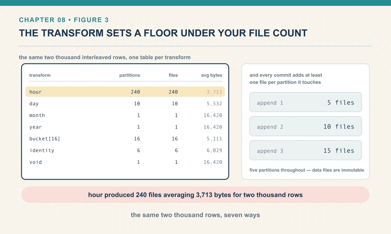
That is the trap, and it is the most common Iceberg mistake I have seen: partition granularity chosen from the query side alone. The rule that actually works is to size partitions so each holds enough data for a sensible file — hundreds of megabytes, not kilobytes. Let statistics handle the finer filtering inside them. A day partition holding 200 MB is healthy. An hour partition holding 3 KB is a bill.
Repairing those small files takes maintenance work, which chapters 11 and 12 measure. Coarser partitions can avoid creating them in the first place.
Replacing one partition
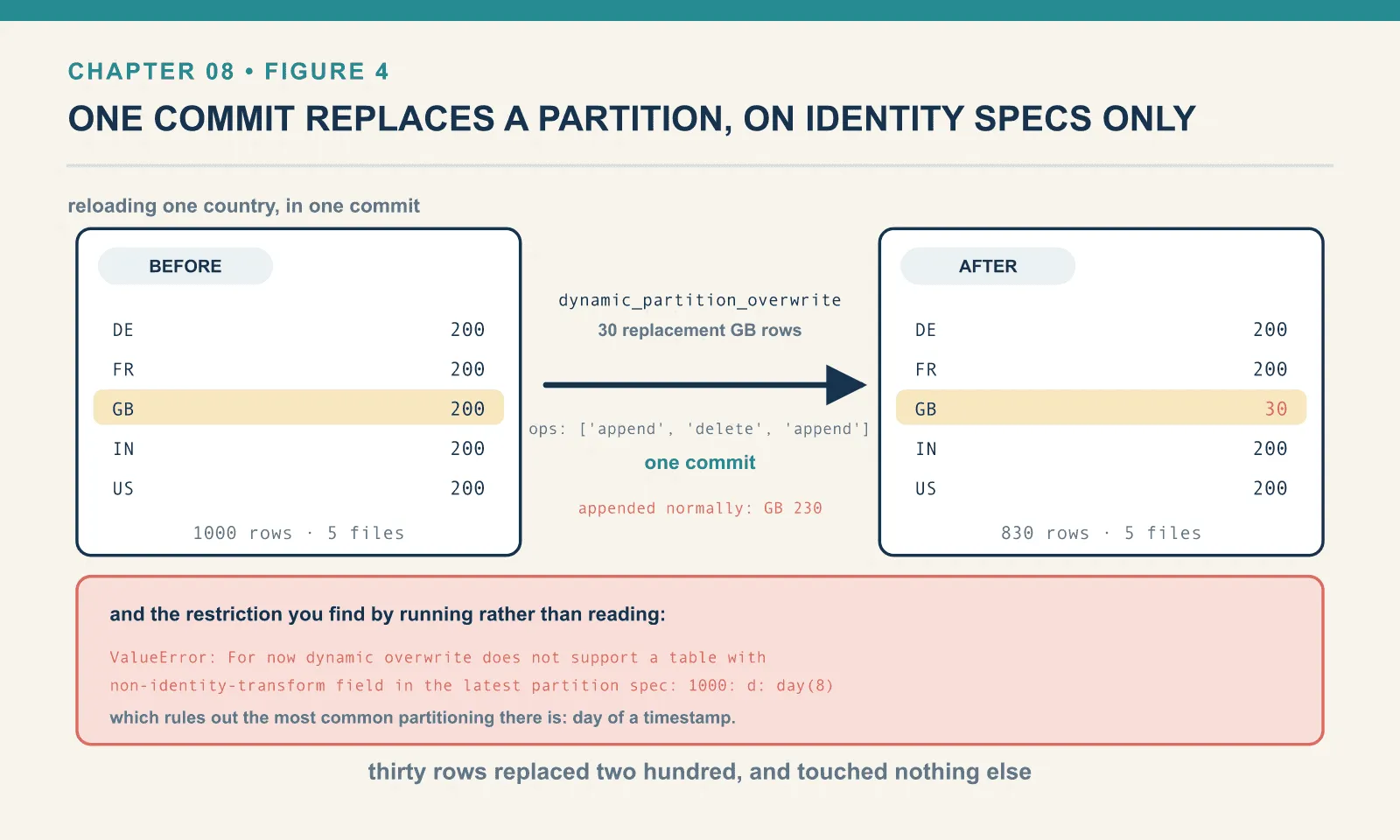
The operation partitioned tables exist to make easy is “reload yesterday”, and PyIceberg has it:
t.dynamic_partition_overwrite(new_rows)before: 1000 rows, 5 files {'DE': 200, 'FR': 200, 'GB': 200, 'IN': 200, 'US': 200}
after : 830 rows, 5 files {'DE': 200, 'FR': 200, 'GB': 30, 'IN': 200, 'US': 200}
ops: ['append', 'delete', 'append']Thirty replacement rows for GB replaced the two hundred that were there, and touched nothing else. The same batch appended normally would have given GB: 230. That is the wrong answer for a reload, and the reason people write a delete-then-insert dance that is not atomic. Here it is one commit, recorded as a delete and an append, published together.
There is a significant restriction, and it is the kind of thing you find by running rather than reading:
ValueError: For now dynamic overwrite does not support a table with
            non-identity-transform field in the latest partition spec: 1000: d: day(8)
PyIceberg 0.11.1’s dynamic_partition_overwrite only works on identity-transform specs. A table partitioned by day(ordered_at) is refused outright, and that is the most common Iceberg partitioning there is. The message is explicit, which is a mercy. The workaround in PyIceberg is an overwrite with a filter that names the day window on the source column. Spark’s INSERT OVERWRITE has no such limitation. This is on the list of things to re-check by version rather than to memorise.
Choosing a spec
A useful spec has to match both the queries and the volume arriving in each write. The measurements above give two checks: how many files a query can skip, and how small the resulting files become.
Partition on the column your queries actually filter. Not the column you think of as the table’s identity. If nobody filters by country, partitioning by country buys nothing and costs a file per country per commit.
Size the partition, not the count. Aim for partitions large enough to hold files in the hundreds of megabytes. Work it out from your daily volume. A table taking a million rows a day probably wants day; one taking a thousand probably wants month; one taking a hundred probably wants no partitioning at all.
Two fields is usually the maximum. A spec of day(ordered_at) plus bucket(16, customer_id) gives you 16 files per day and answers both time-range and customer queries. A spec of day plus country plus channel plus status gives you a Cartesian product of tiny files, and a table that is slow in a way nobody will attribute to the spec.
Do not partition a small table. Under a few gigabytes, column statistics do this job perfectly well. Every partition you add is a floor on your file count.
And do not partition on something that changes. A partition value is derived at write time from the row’s own data. If status moves from placed to shipped, a row partitioned by status has to be physically moved, which means a rewrite. Partition on facts, not on state.
Final thoughts
Hidden partitioning is a small idea with an unusually good ratio of benefit to complexity. The table stores a function; the planner applies it to your predicates; the physical layout stops being something a query author has to know. What used to be a class of silent, expensive mistakes becomes impossible to make, because the mistake required a partition column and there isn’t one.
What it does not do is choose the function for you. Everything measured in this chapter — 240 files of 3.7 KB, a range query that could not use a bucket, fifteen files from three appends — came from a spec that was wrong for its data. None of it came from anything the format did badly.
Which raises the obvious question, and it is the one Hive could never answer. You partitioned by day when the table took a thousand rows a day; it now takes ten million. What do you do with the two years of files already written under the old spec?
Comments