Four Books and a Catalog

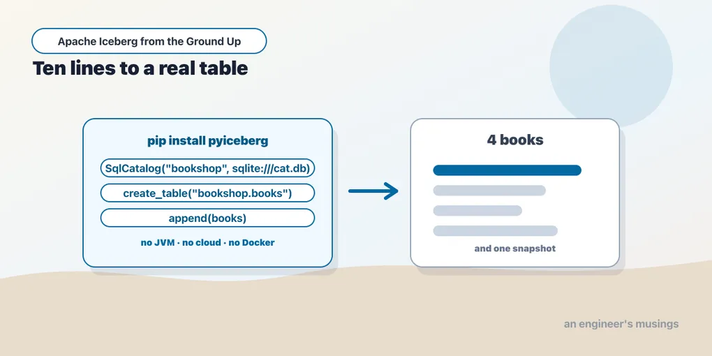
The last chapter argued that a folder is not a table. This one makes a table, and it takes about ten lines.

That is worth stating plainly. Most Iceberg introductions open with a Spark shell, a JVM, a jar coordinate and a Docker Compose file, and a good number of readers never make it past that to the part where the format does something. None of it is necessary. Everything in this chapter runs on a laptop with one install and a local directory:

pip install "pyiceberg[sql-sqlite,pyarrow]"

Pinned versions for this book: PyIceberg 0.11.1, PyArrow, Python 3.13, plus DuckDB 1.5.5 and pandas where they appear.

If you would rather not assemble the environment by hand, the companion repository iceberg-bookshop pins all of it — make venv and you have exactly what this book was written against.

We build the bookshop here, and it carries the rest of the book: books, orders, customers. It starts with four books.

You cannot skip the catalog, even alone

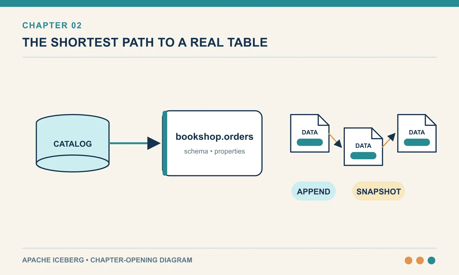
Even a table on a laptop needs an authoritative answer to which files are current. The catalog supplies it: a table name resolves to one metadata file, and a commit swaps that pointer atomically. Iceberg defines the interface; you bring an implementation.

For a laptop, the implementation is a SQL database, and SQLite counts:

from pyiceberg.catalog.sql import SqlCatalog

catalog = SqlCatalog(
    "bookshop",
    uri="sqlite:///cat.db",
    warehouse="file:///abs/path/wh",
)

Two arguments and a name. The uri is where the pointer lives; the warehouse is where data files go. This is a real, spec-conforming catalog rather than a toy. The same SqlCatalog class runs against Postgres in production, and SQLite is only the backend. Chapter 4 opens it up and reads every column; chapter 5 swaps it for a catalog server.

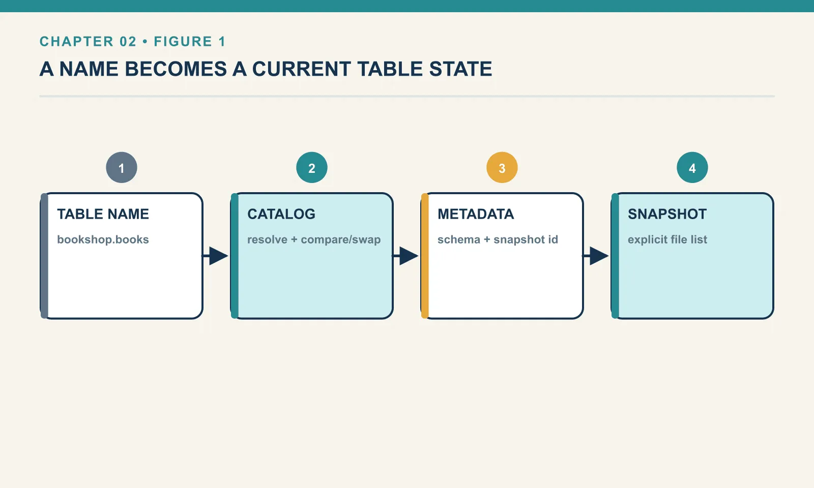
One thing about that first argument, because it costs people an afternoon. The catalog’s name is part of its identity, not a label. I later reconnected to the same SQLite file with SqlCatalog("b", ...) instead of SqlCatalog("bookshop", ...) and got:

pyiceberg.exceptions.NoSuchTableError: Table does not exist: bookshop.books

The file was right there, the table was right there. But the catalog stores its own name alongside every table. A different name is therefore a different catalog that happens to share a database file, and it is empty. There is no warning, because nothing is wrong: you asked an empty catalog what it contained, and it told you.

Namespaces, then a table

A namespace is a container for tables. Create one:

catalog.create_namespace("bookshop")

  before: []
  after : [('bookshop',)]

Create it twice and Iceberg objects rather than shrugging:

NamespaceAlreadyExistsError: Namespace bookshop already exists

Now the table. The quickest route is to hand PyIceberg an Arrow table and let it derive the schema:

import pyarrow as pa

books = pa.table({
    "book_id": pa.array([1, 2, 3, 4], pa.int64()),
    "title":   ["Dune", "Neuromancer", "Blindsight", "Anathem"],
    "author":  ["Herbert", "Gibson", "Watts", "Stephenson"],
    "genre":   ["scifi", "cyberpunk", "scifi", "scifi"],
    "price":   pa.array([9.99, 7.50, 6.25, 12.00], pa.float64()),
})

t = catalog.create_table("bookshop.books", schema=books.schema)

identifier: ('bookshop', 'books') | format_version: 2
table {
  1: book_id: optional long
  2: title: optional string
  3: author: optional string
  4: genre: optional string
  5: price: optional double
}
current_snapshot: None

Every field has a number. 1: book_id, 2: title, and so on. Those are field IDs, and they are how Iceberg tracks a column through renames and reordering. They are why a rename here is safe when the same rename against a folder of Parquet is the trap we hit in chapter 1. Chapter 7 is entirely about them.

format_version: 2. Not 3, even though version 3 has been production-ready since May 2026. The default is deliberate, and chapter 19 covers what v3 adds and why the upgrade is not automatic.

current_snapshot: None. The table exists and has no data, and those are separate facts. A table is a name, a schema, and a pointer — the pointer just does not point at any data yet.

Append, and the table acquires a history

t.append(books)

rows: 4 | snapshot: 88002193332962349

That is a commit. Four rows landed, and the table now has a snapshot with an id — a name for the state it is in. Nothing about that id is cosmetic. Chapter 6 uses it to read the table as it was, and chapter 1 used its ancestor to roll a bad refresh back.

Reading it, four ways

The scan API is where you will spend most of your time:

t.scan().to_arrow()                                   # 4 rows
t.scan(selected_fields=("title", "price")).to_arrow()  # ['title', 'price']
t.scan(row_filter="genre == 'scifi'").to_arrow()       # 3 rows
t.scan().to_pandas()                                   # a DataFrame

to_arrow  : 4 rows
selected  : ['title', 'price']
filtered  : 3 rows
to_pandas : ['book_id', 'title', 'author', 'genre', 'price']
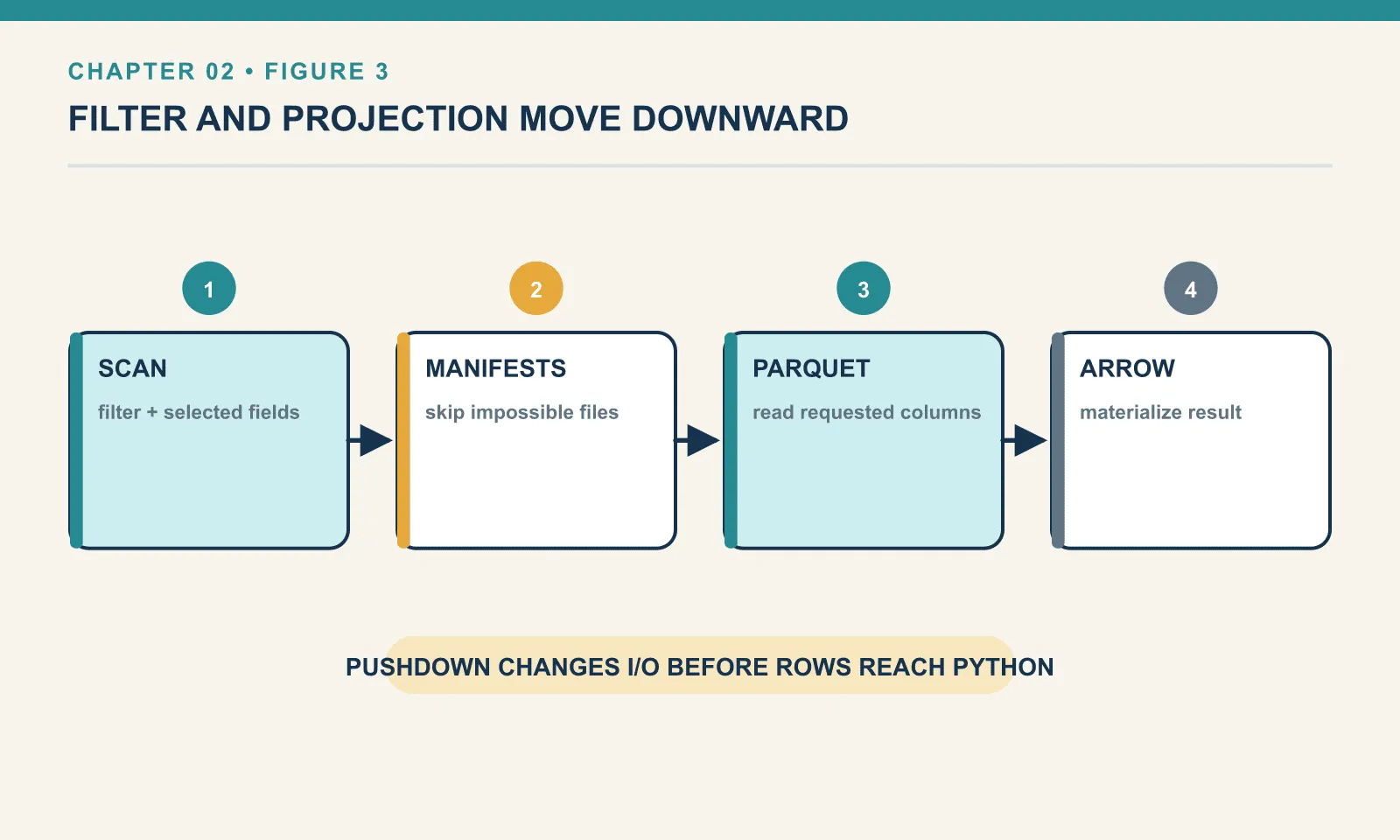
duckdb    : [(4, 8.94)]

The projection and the filter are not conveniences applied after loading. Iceberg pushes both down. The filter is evaluated against per-file statistics to skip whole files before any are opened, and the projection limits which Parquet columns are read. On four rows this is invisible. On four hundred million it is the difference between a query and a bill.

The last line is DuckDB aggregating the Arrow that PyIceberg produced, for an average price of 8.94. Arrow lets a second engine work with this result without an export step; chapter 15 develops the broader multi-engine case.

Loading from a file, which is how it really starts

Handing create_table a hand-built Arrow table is the tutorial version — in practice the first table comes from a file. The shape is the same: read it with Arrow, derive the schema, append.

import pyarrow.csv as pacsv

cust = pacsv.read_csv("customers.csv")
ct = catalog.create_table("bookshop.customers", schema=cust.schema)
ct.append(cust)

inferred: [('customer_id', 'int64'), ('name', 'string'), ('country', 'string')]
customers: 3 rows

Arrow’s CSV reader did the type inference, and Iceberg took what it was given. That is convenient, and it is also the weak point. The schema of your table is now whatever a type sniffer guessed from the first few thousand rows of one file. Two chapters from now that schema is a contract every future write must satisfy. If the table matters, read the inferred types out loud before you accept them, or declare the schema by hand.

Five ways your first table quietly misbehaves

Creating the table was easy; deciding what writes it should accept takes more care. The inferred schema permits several changes that a producer might make by accident, and only two of the failures below raise an error.

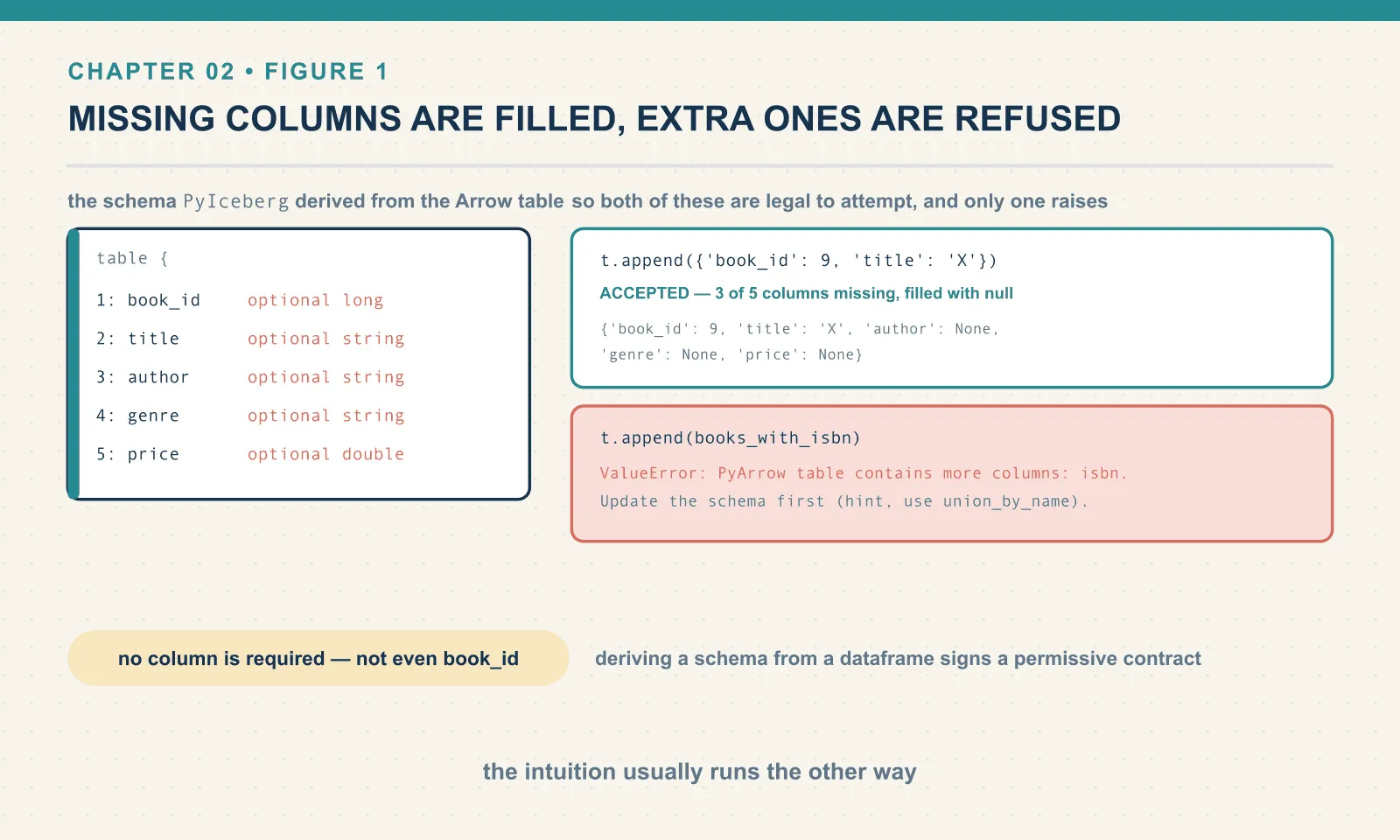
Everything is optional. Look again at the schema Iceberg derived: every field says optional. Arrow’s default nullability came straight through, so no column is required. That includes book_id, which is obviously a key. If you want required columns you must declare the schema explicitly rather than deriving it:

from pyiceberg.schema import Schema
from pyiceberg.types import NestedField, LongType, StringType

Schema(
    NestedField(1, "id",   LongType(),   required=True),
    NestedField(2, "name", StringType(), required=False),
)

A partial append succeeds, silently. Because every column is optional, appending a table that is missing most of them is legal:

t.append(pa.table({"book_id": pa.array([9], pa.int64()), "title": ["X"]}))

No error. The row lands, and the missing columns are filled with nulls:

{'book_id': 9, 'title': 'X', 'author': None, 'genre': None, 'price': None}

A pipeline that drops three columns after an upstream change will not fail. It will write nulls, on schedule, until somebody notices the average price moving.

Types get promoted. Appending book_id as int32 against a schema that says long also succeeds. Iceberg accepts the widening and stores int64. That is correct and useful, and it is one more mismatch that does not announce itself.

There are no primary keys. After the two appends above, the table holds nine rows, and two of them have book_id 9:

{'book_id': 9,  'title': 'X',    'author': None, ...}
{'book_id': 9,  'title': 'Dune', 'author': 'Herbert', ...}

Iceberg has no unique constraint, no primary key and no ON CONFLICT. It is a table format, not a database. Uniqueness is your pipeline’s job, and upsert and MERGE INTO (chapters 10 and 16) are how you enforce it deliberately.

An unknown column, on the other hand, is refused. This is the one asymmetry:

ValueError: PyArrow table contains more columns: isbn.
            Update the schema first (hint, use union_by_name).

Missing columns are filled; extra columns are rejected. Worth internalising, because the intuition usually runs the other way.

And when you do declare a field required, PyIceberg enforces it — with the clearest error message in the library, a field-by-field diff:

┏━━━━┳━━━━━━━━━━━━━━━━━━━━━━━━━━┳━━━━━━━━━━━━━━━━━━━━━━━━━━┓
┃    ┃ Table field              ┃ Dataframe field          ┃
┡━━━━╇━━━━━━━━━━━━━━━━━━━━━━━━━━╇━━━━━━━━━━━━━━━━━━━━━━━━━━┩
│ ❌ │ 1: id: required long     │ Missing                  │
│ ✅ │ 2: name: optional string │ 2: name: optional string │
└────┴──────────────────────────┴──────────────────────────┘

The lesson is not that PyIceberg is careless. It is that an all-optional schema is a permissive contract, and deriving your schema from a DataFrame silently signs one. Declare the schema when the table matters.

Changing data, and the trap that was waiting

We have a table with two rows sharing book_id 9. The obvious fix is an upsert, and PyIceberg has one:

t.upsert(fix, join_cols=["book_id"])

UpsertResult(rows_updated=2, rows_inserted=0)

Two rows updated is the warning here. Upsert matched on book_id, found both rows with id 9, and updated both. The table now holds two identical copies of Hyperion:

{'book_id': 9, 'title': 'Hyperion', 'author': 'Simmons', 'genre': 'scifi', 'price': 8.75}
{'book_id': 9, 'title': 'Hyperion', 'author': 'Simmons', 'genre': 'scifi', 'price': 8.75}

The duplicate did not go away. It got twice as convincing.

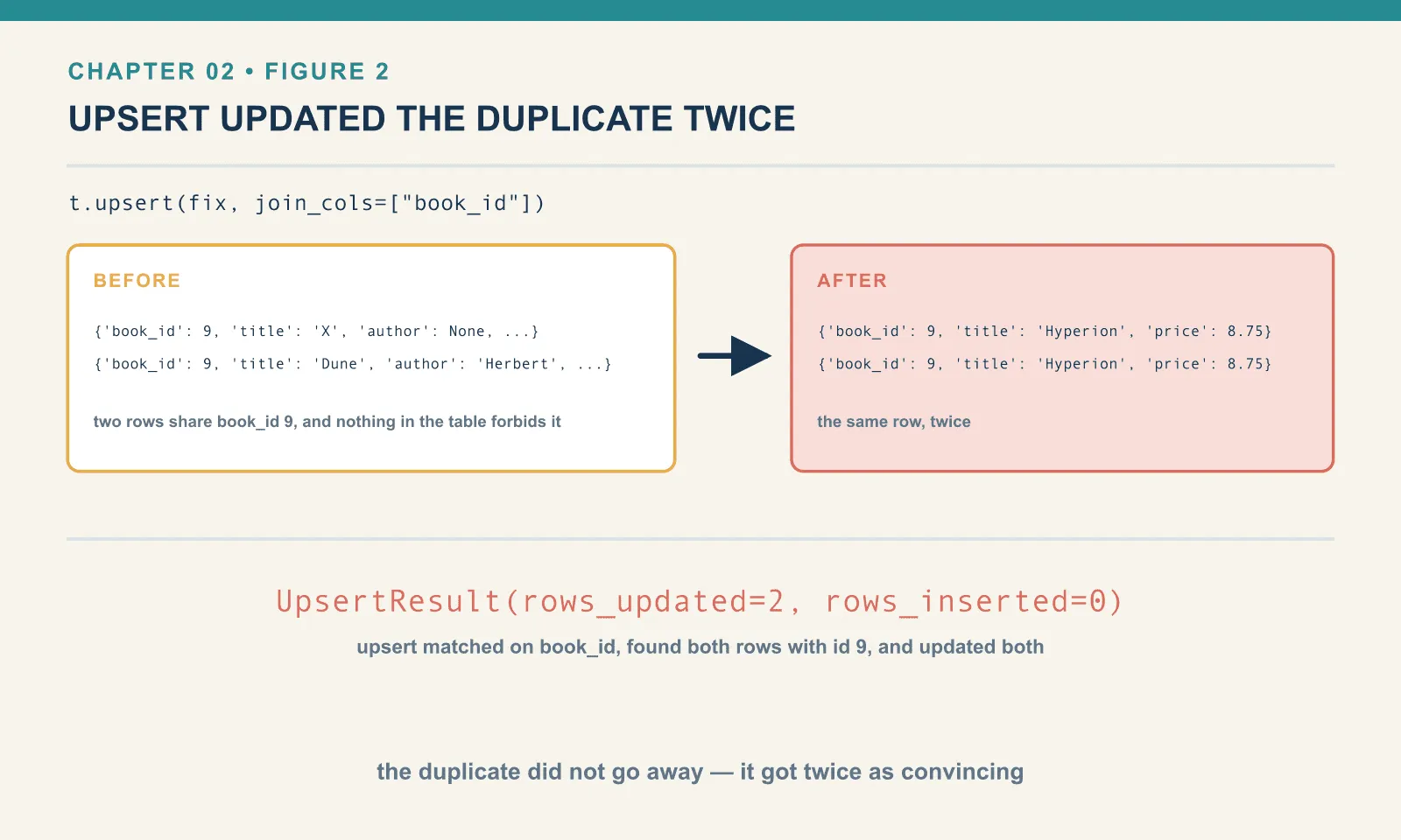
This is the payoff of “there are no primary keys.” Upsert is exactly the tool people reach for to impose uniqueness, and it cannot. join_cols tells Iceberg how to match rows. It does not assert that the match is unique, and nothing anywhere in the table does. Uniqueness has to hold before the upsert, not after it. If duplicates can enter your table, deduplicate on the way in.

Deleting is simpler, and takes a row filter rather than a row set:

t.delete("genre == 'cyberpunk'")

rows: 7

Two rows gone. No warning was emitted for this particular delete: PyIceberg only complains about merge-on-read when it has to fall back to it. How a delete is physically carried out is chapter 10’s subject. For now the useful mental model is that delete takes a predicate, not a list of rows. It is also a commit like any other: it produces a snapshot, and chapter 6 can put it back.

The rest of the scan API

Four more things you will want early:

t.scan(limit=2).to_arrow()            # 2 rows
t.scan().to_polars()                  # (7, 5)
t.scan().to_arrow_batch_reader()      # RecordBatchReader, first batch: 2 rows
list(t.scan().plan_files())           # 3 file tasks

to_polars matters if Polars is your dataframe library. to_arrow_batch_reader matters when the result does not fit in memory, since it streams rather than materialising.

plan_files is the interesting one. It returns the file tasks the scan resolved to — the actual list of data files this query will open, after pruning. Three tasks here for three data files, because nothing pruned them. Put a selective filter on it and the count drops, so you see the pruning rather than infer it from a stopwatch. It is the cheapest window into how Iceberg decides what to read, and chapter 8 uses it to prove hidden partitioning works.

Properties, and catalogs for tests

Tables carry a property bag, empty by default:

with t.transaction() as tx:
    tx.set_properties({"owner": "bookshop-team",
                       "write.parquet.compression-codec": "zstd"})

properties: {}                                             # before
{'owner': 'bookshop-team', 'write.parquet.compression-codec': 'zstd'}   # after

Two kinds of thing live in there and it pays to know which is which. owner is yours, arbitrary, and Iceberg never reads it. But write.parquet.compression-codec is a reserved property the writers actually obey. The write.* namespace controls file sizes, compression, delete mode and more. It is where a lot of chapter 11 and 12’s tuning ends up living.

For tests you often want a catalog with no filesystem footprint at all:

from pyiceberg.catalog.memory import InMemoryCatalog
mc = InMemoryCatalog("test", warehouse="/tmp/mem")

in-memory rows: 3 | type: InMemoryCatalog

Same interface, nothing to clean up. It is the right default for unit tests of code that talks to a catalog.

Dropping a table does not delete anything

Removing a table name and reclaiming its storage are separate operations. A drop shows the difference:

catalog.drop_table("bookshop.strict")

files in warehouse before: 37 after: 37 -> files left behind
tables now: [('bookshop', 'books'), ('bookshop', 'customers')]

The table is gone from the catalog. Every one of its files is still on disk. Thirty-seven before, thirty-seven after.

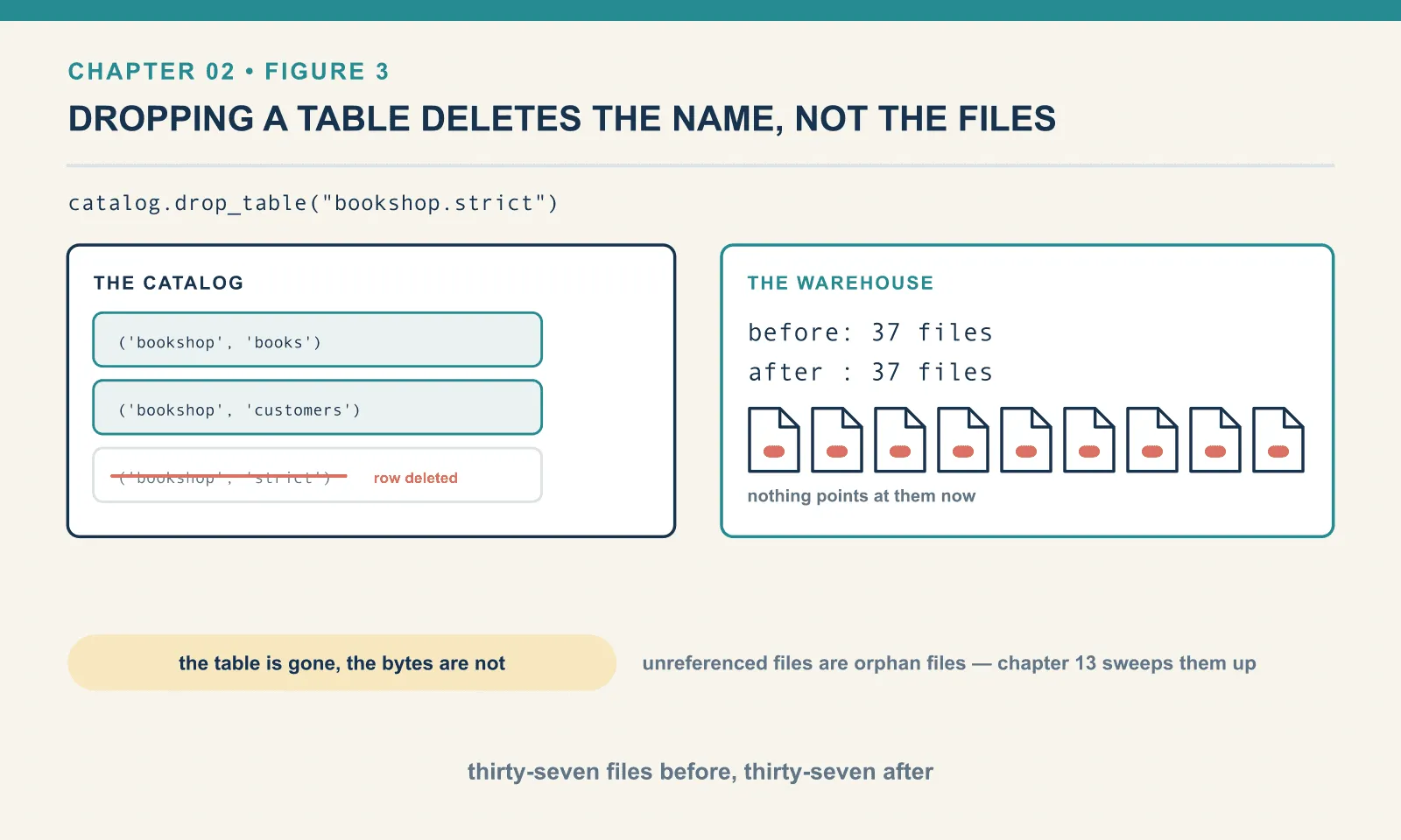
That is consistent rather than careless. The catalog’s job is the pointer, and dropping a table means forgetting the pointer. The data files are not referenced by anything now, which makes them precisely orphan files — the thing chapter 13 spends a section cleaning up. On a laptop it is thirty-seven files. On a warehouse where somebody drops and recreates a table nightly, it is a storage bill that grows forever and a directory nobody dares delete by hand.

Some catalogs support a purge variant that deletes the data too. Check whether yours does, and whether you want it to, before you need it rather than after.

One commit, or two? The transaction API

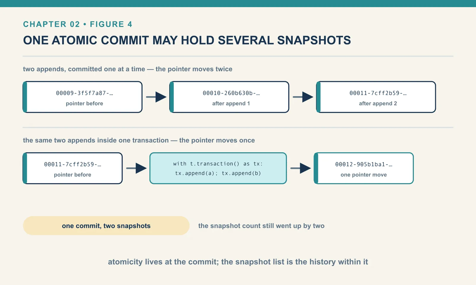
Every operation so far committed on its own. Two appends means two commits, and you can watch the catalog pointer move twice:

pointer before : 00009-3f5f7a87-….metadata.json
after append 1 : 00010-260b630b-….metadata.json
after append 2 : 00011-7cff2b59-….metadata.json

Group them in a transaction and they commit together:

with t.transaction() as tx:
    tx.append(batch_a)
    tx.append(batch_b)

after transaction : 00012-905b1ba1-….metadata.json

One pointer move for two appends. Nobody can observe a state where the first landed and the second did not.

Now the part I got wrong before running it. I assumed the transaction would also collapse the two appends into one snapshot. It does not — the snapshot count still went up by two. So the precise rule is:

A transaction is one atomic commit that may contain several snapshots.

Atomicity lives at the commit, and the snapshot list is the history within it. Chapter 1 found the same shape by accident, where a single overwrite recorded a delete and an append while readers observed one change. Same mechanism, stated properly.

The practical consequence is for writers. If your job produces ten batches, ten separate append calls mean ten commits, ten chances to collide with another writer, and ten pointer swaps. One transaction means one. It does not, however, mean one file. Batching commits is not the same as batching data, which is why chapter 11’s small-files problem survives this trick.

What you have now

Every commit in this chapter — each append, the upsert, the delete, the property change — produced a snapshot, and most produced a data file. One append, one snapshot, one file is the tidy version of that. It is also the seed of the small-files problem that chapter 11 measures. A table written a row at a time ends up with a file per row and metadata that dwarfs it.

You have a real Iceberg table. It has a schema with stable field IDs, a history you can query, and atomic commits. Its physical layout is one other engines can read without asking you anything. It cost one pip install and a directory.

The wh/ folder now contains rather more than three Parquet files. Those additional files hold the schema, history and file lists that made these operations possible. Chapter 3 opens them and accounts for each one.

Next: Anatomy of a Table