What the Engine Refuses to Read
Columnar storage, vectorized execution and morsel parallelism, measured — including a query whose EXPLAIN ANALYZE plan is completely empty, and an index that the planner declined to use in every single case.
If you came through the SQL performance series, you have a working model of how a database gets fast, and it is a good one. Data lives in row-shaped pages. Scanning is expensive, so you build an index. The planner picks between a sequential scan and an index scan based on statistics. Tuning is largely the art of giving it better options.
Almost none of that applies here.
DuckDB has no index on the table you are about to see, will not build one that helps, and answers a point lookup in 20 million rows in 0.6 milliseconds anyway. That is not a smaller version of the same design. It is a different one, and this chapter is about what replaces the parts you know.
Everything here was run against DuckDB 1.5.5 on a 20-million-row Parquet file — 394 MB, eight columns, on a 16-thread laptop.
The unit of storage is a column
Start with the claim from chapter 1 and make it precise. In a row store, a row’s fields sit next to each other on disk. Reading one field means reading the page that contains it, which means reading every other field of every row on that page.
In a column store, each column is stored separately. Reading one column touches only that column’s bytes. The rest of the table is not on the way to anything.
The consequence is measurable, and you can measure it by counting columns:
select sum(bytes) from 'big/hits.parquet';                                  -- 1 column
select sum(bytes), sum(duration_ms), sum(status) from 'big/hits.parquet';   -- 3 columns
-- and one summing something from all eight
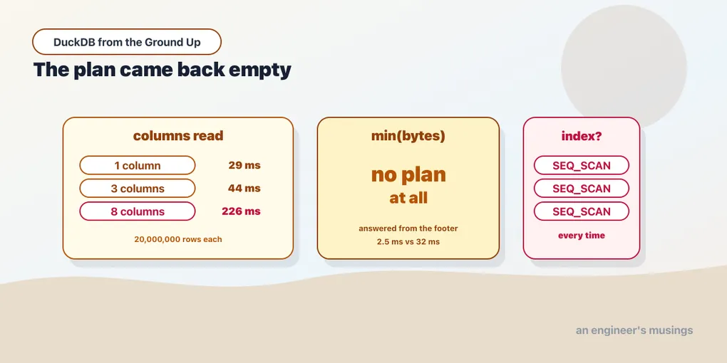
1 column : 29 ms
3 columns : 44 ms
8 columns : 226 msSame file, same 20 million rows, same aggregate shape. The only variable is how many columns the query needs, and the time tracks it almost linearly. What you do not select, you do not pay for.
That is the sentence to hold onto, because it inverts a habit. In a row store, select * on a wide table costs about what select one_column costs, so nobody thinks about it. Here, select * is the most expensive query you can write.
Reading the plan
EXPLAIN ANALYZE shows the pruning as a property of the scan itself. From the query in chapter 5, over five files:
┌─────────────┴─────────────┐
│         TABLE_SCAN        │
│    ────────────────────   │
│         Function:         │
│        PARQUET_SCAN       │
│                           │
│        Projections:       │
│       client.country      │
│                           │
│    Filters: status=200    │
│    Total Files Read: 5    │
│                           │
│        285,716 rows       │
│           0.01s           │
└───────────────────────────┘
Three things are happening in that one node, and all three are the engine deciding not to read something.
Projections: client.country — the table has nine columns and the scan lists one. This is projection pushdown, and note what it pushed down: not client, but client.country. The client column is a struct with country and city fields, and only the country field was read. Pushdown reaches inside nested types.
Filters: status=200 — the filter did not happen above the scan, it happened inside it. 500,000 rows in the files, 285,716 rows out of the scan node. The rows that failed the filter were never handed upward.
Total Files Read: 5 — file-level pruning, which is where the 1/5 from chapter 5 appears when the filter is on a partition column.
Compare that with the plan you would read in a row store. There the scan node emits rows, and separate Filter and Projection nodes discard work that has already been done. Here the discarding is the scan.
The query with no plan at all
Now the result that makes the point better than any of the above. Two nearly identical queries:
select min(bytes) from 'big/hits.parquet';
select sum(bytes) from 'big/hits.parquet';
min(bytes) : 2.5 ms
sum(bytes) : 32.2 msThirteen times apart, for one column and one aggregate each. Ask EXPLAIN ANALYZE about the slow one and you get what you expect:
│         TABLE_SCAN        │
│     Projections: bytes    │
│      20,000,000 rows      │
│           0.40s           │
Ask it about the fast one and you get this:
┌────────────────────────────────────────────────┐
││              Total Time: 0.0000s             ││
└────────────────────────────────────────────────┘
There is no plan. No scan node, no aggregate node, nothing. The query tree is empty because no query ran.
Parquet files carry per-row-group statistics, including the minimum and maximum of every column. min(bytes) over the whole file is the minimum of 163 per-group minimums, and all 163 of those numbers are in the footer. The optimizer answered the question from metadata and never opened a data page.
You can see the same statistics directly:
select row_group_id, row_group_num_rows, stats_min, stats_max
from parquet_metadata('big/hits.parquet') where path_in_schema='id' limit 3;
(0, 122880, '0', '122879')
(1, 122880, '122880', '245759')
(2, 122880, '245760', '368639')163 groups of 122,880 rows, each carrying the range of every column it holds. These are zone maps, and they are the reason the next section goes the way it does.
The index that never got used
Here is the reflex the Postgres book installs. A point lookup on 20 million rows sounds slow, so:
create index idx on hits(id);It builds in 1.4 seconds. Then, on a native DuckDB table:
point lookup, no index :  0.60 ms
point lookup, w/ index :  0.57 ms
No improvement, and the reason is in the plan:
explain select bytes from hits where id = 12345678;SEQ_SCANSEQ_SCAN, with the index sitting right there. I tried the same thing several ways: an equality on a clustered column, a range over a million rows, and an equality on user_id, which cycles every 50,000 rows and so is about as unclustered as a column gets. Every plan came back SEQ_SCAN. On the unclustered column the indexed run was, if anything, marginally slower than the unindexed one, and both were within noise of each other.
The lookup does not need the index. id ranges from 0 to 19,999,999, the zone maps say group 100 holds 12,288,000 through 12,410,879, and 12,345,678 is inside exactly one group. DuckDB reads one row group of 122,880 values and scans it. That is the 0.6 milliseconds, and it happens with no index because the statistics were already there.
The honest scope of that claim: DuckDB does have indexes, they are ART indexes, and their real job is enforcing PRIMARY KEY and UNIQUE constraints. They are not a query-acceleration tool you reach for when something feels slow. Every plan I looked at on this table preferred a scan, and none of them were wrong to.
So when a DuckDB query is slow, “add an index” is not the first move. It is usually not a move at all. The levers are the ones in the rest of this chapter: read fewer columns, filter earlier, give the data a layout whose zone maps are selective.
Vectorized, which is neither of the obvious options
There are two obvious ways to run a query, and both are bad.
Row at a time is what a traditional interpreter does: for each row, walk the expression tree, call a function per operator. Correct, flexible, and dominated by interpretation overhead — you spend more time deciding what to do than doing it.
Whole column at a time is what early column stores did: materialise the full result of every operator. Very little overhead per value, but a 20-million-row intermediate has to live somewhere, and it will not be in cache.
DuckDB takes the middle: it processes vectors — batches of roughly a couple of thousand values from one column. Big enough that the per-batch overhead disappears into the batch. Small enough that the batch fits in CPU cache, so the next operator reads it out of L1 rather than RAM.
That is the design. Here is what it costs to leave it. The same arithmetic on 2 million values, once as SQL and once as a Python function registered as a UDF:
def scale(x): return x * 2 + 1
con.create_function('py_scale', scale, ['BIGINT'], 'BIGINT')
native SQL sum(bytes*2+1) : 11 ms
python UDF sum(py_scale) : 378 msThirty-four times slower for identical arithmetic. Nothing about the maths changed. What changed is that every value crossed out of the vectorized engine into the Python interpreter and back, one at a time, and the batching stopped applying.
This is the most practical thing in the chapter. When a DuckDB query is unexpectedly slow, the first question is not “what index is missing” but “where did I leave the engine?” A Python UDF, a row-by-row loop over fetchall(), a per-row call into another library — each of those is a place where the vectors get unpacked. Express it as SQL and it stays in the engine.
Parallelism, and where it stops
Vectors also make parallelism easy: hand different threads different batches. DuckDB calls the unit a morsel, and the same query at different thread counts:
threads=1   group by country :      98 ms
threads=2   group by country :      50 ms
threads=4   group by country :      30 ms
threads=8   group by country :      19 ms
threads=16  group by country :      18 ms
One to two halves it. Two to four nearly halves it again. Four to eight, again. Eight to sixteen buys 1 millisecond.
The flattening is not a DuckDB limit, it is the machine. This laptop has eight physical cores, so threads 9 through 16 are hyperthreads sharing execution units with threads 1 through 8. Scaling tracks real cores, then stops.
Two things follow. First, this is parallel by default — nobody configured anything, and threads came up at 16 on its own. Second, the whole machine is the unit of scaling. A cloud warehouse scales by adding nodes, and you pay per node. DuckDB scales by using the cores you already have, and eight cores is an ordinary laptop. That is a large fraction of the “we need a cluster” cases, answered by a default.
There is one consequence of parallel-by-default that catches people, and it is worth knowing before it does. Floating-point addition is not associative, so a sum split across threads and recombined can land on a slightly different value depending on which thread finished first. Running the same average over this dataset eight times:
20.995000000000303
20.994999999998836
20.99499999999992
…
Same data, same query, same engine — the last few digits move. Pin threads=1 and it becomes perfectly repeatable, which is how you confirm the cause rather than guessing at it.
This is not a DuckDB bug and every parallel engine has it. It matters in two places: never compare two float aggregates with =, and if you are writing a test or a book that pastes an average, round it to a precision the arithmetic can actually guarantee. Integer aggregates — count, sum over integers — are unaffected.
When to stop querying files
Chapter 5 said to query Parquet in place while exploring and materialise once the access pattern settles. Here is the number behind that advice. The same 20 million rows, as a Parquet file and as a native DuckDB table:
parquet file sum(bytes)    :      33 ms
native table sum(bytes)    :       5 ms
parquet : 394.5 MB
duckdb : 207.1 MBSix and a half times faster, in a little over half the space.
DuckDB’s own storage format can assume things Parquet cannot. Parquet is an interchange format, so it is conservative — anything must be able to read it. DuckDB’s format is read by exactly one engine, so it can compress per column with whatever scheme fits that column’s data, and lay it out for its own scanner.
Take the size number with some salt: this file is synthetic and repetitive, which flatters any compressor, and a real dataset may land either way. The speed gap is the more reliable finding, and it is the one that should drive the decision. Explore against files. When you find yourself running the same query for the third time, load it.
Final thoughts
Every result here is the engine avoiding work rather than doing it faster. It reads one column of eight. It filters inside the scan. It answers min() from a footer and never plans a query. It prunes 162 of 163 row groups from statistics it already had, which is why an index changed nothing.
That last one is the piece most worth carrying, because it is a reflex you have to actively unlearn. In a row store, “this filter is slow” and “this needs an index” are nearly the same sentence. Here they are unrelated. The plan said SEQ_SCAN every time, and every time it was right.
The two levers that do work: read fewer columns, and stay inside the vectorized engine. One is a select list. The other is the difference between 11 milliseconds and 378.
Next: When It Doesn’t Fit — what actually happens at the memory limit, where the spill goes, and which operations degrade gracefully rather than failing.
Comments