The Star Schema

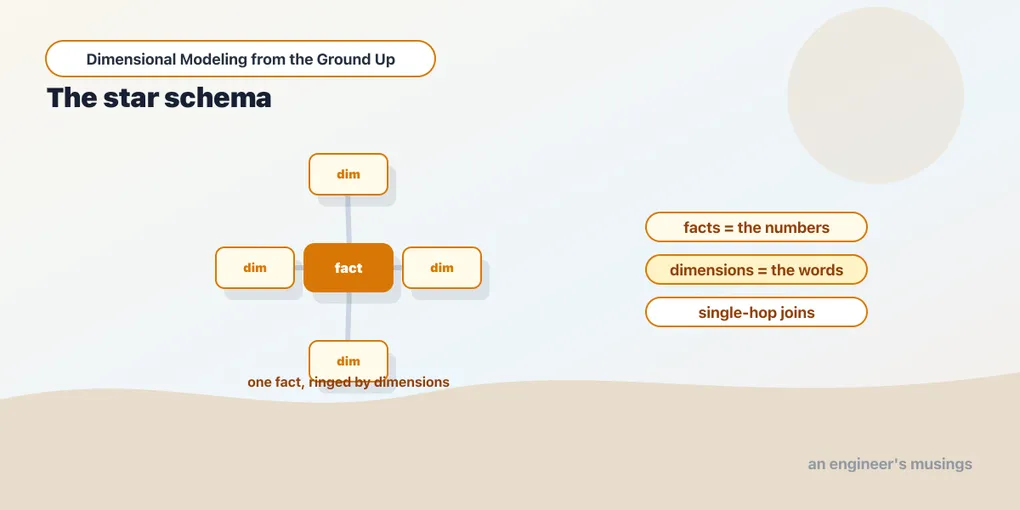
Draw the bookshop’s remodeled warehouse and it looks like a star. One table sits in the middle, and a handful of others ring it, each connected by a single foreign key. That picture has a name — the star schema — and it’s the destination for almost everything in dimensional modeling.

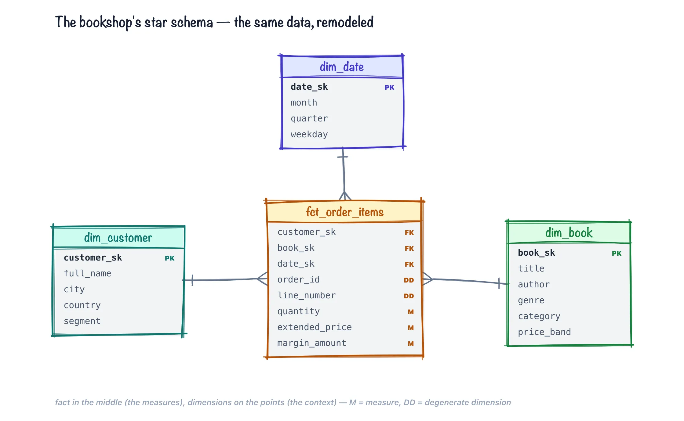
The table in the center is a fact table. It holds the measurements — the numbers you sum, count, and average. Here that’s the order lines: how many copies, at what price, for how much. The tables on the points are dimension tables. They hold the descriptive context — the words you slice those numbers by. Who bought (dim_customer), what they bought (dim_book), and when (dim_date). The fact table carries a foreign key to each one and almost nothing else.

The split is the whole idea. Facts are what you measure; dimensions are what you measure it by. Say a business question out loud and it sorts itself: “revenue by genre by month” — revenue is a fact, genre and month are dimensions. Nearly every analytics question has that shape, which is why nearly every warehouse has this one.

Why a star and not the source

Go back to the five-join question from the last post. Against the normalized source it needed order_items → orders → books and beyond, plus the arcane knowledge that revenue is quantity * unit_price and cancelled orders don’t count. Against the star it’s this:

select
    d.month,
    b.genre,
    sum(f.extended_price) as revenue
from fct_order_items as f
join dim_book  as b on f.book_sk = b.book_sk
join dim_date  as d on f.date_sk = d.date_sk
group by 1, 2

Same answer, different world. Revenue is a column that already means revenue — the quantity * unit_price math and the cancelled-order filter were settled back in staging, so they’re not in this query and they can’t be gotten wrong here. Every join is fact-to-dimension on a single key; there are no chains to route through and no order to memorize. And the shape generalizes: swap dim_book.genre for dim_customer.region and you’ve got revenue by region by month with no new joins to learn. That predictability is the payoff. In the source schema every question is a small research project; in the star it’s the same join pattern with different columns.

The pattern is worth stating as a template, because it’s the only one the star ever asks you to learn:

select   <dimension attributes>,
         <aggregates of fact measures>
from     <fact>
join     <dimension> on <single key>   -- repeat per dimension used
where    <dimension attribute filters>
group by <dimension attributes>

Every question the bookshop will ask of this star is an instantiation. Units by author: aggregate quantity, attribute author. Revenue from premium-band books in Q2: filter price_band and quarter, aggregate extended_price. Average order value by region: two aggregates (sum(extended_price), count(distinct order_id)) and a division. BI tools understand this template natively — point one at a star, declare which table is the fact, and the drag-and-drop interface generates exactly these queries, which is no coincidence: the star schema and the BI query generator co-evolved, and the tools still assume the shape.

The predictability has a name worth knowing early: the measures in a well-built fact table are additive — safe to sum() across any combination of dimensions. sum(extended_price) by genre, by region, by month, or across everything at once all produce true numbers, which is what lets an analyst remix the query above endlessly without re-deriving anything. Not every number the business cares about has that property (an inventory level doesn’t sum across days; a margin percentage doesn’t sum across anything), and designing around the exceptions is a chapter of its own — the fact tables post takes the taxonomy apart. For now, the design instinct: a star works best when the fact’s columns are numbers that add.

The rules of the shape

The star’s simplicity is enforced by two structural rules, and everything else in this series is downstream of them.

Rule one: every fact-to-dimension relationship is many-to-one. Millions of fact rows point at dim_book; each fact row points at exactly one book row. That direction is load-bearing in both directions. The dimension’s key must be unique — one row per book, no duplicates, ever — because a fact row that matches two dimension rows gets duplicated by the join, and every sum() over it silently inflates. And the fact’s foreign key must always resolve — every book_sk in the fact exists in the dimension — or rows quietly vanish from inner joins. Uniqueness on one side, referential integrity on the other: those two properties are the star, and both are testable, which is where dbt comes back into the picture below.

It’s worth seeing the failure concretely once, because it’s the quietest bug in analytics. Suppose a botched load leaves dim_book with two rows for book 101:

fct_order_items                      dim_book
order_id  book_sk  extended_price    book_sk  title
1001      abc101   15.00             abc101   Dune
1001      abc101   15.00   ◀──┐      abc101   Dune      ← duplicate row
1002      abc101   30.00      │
                              └── each fact row matches BOTH dim rows

Join the fact to that dimension and every one of the three fact rows matches twice, so the join emits six rows and sum(extended_price) reports 120.00 instead of 60.00. Nothing errors. No query fails. Revenue for Dune is exactly double, revenue for every other title is correct, and the dashboard total is wrong by an amount nobody can eyeball. The uniqueness rule isn’t tidiness; it’s the only thing standing between a duplicated dimension row and a silently inflated number on every report that touches it.

Rule two: one star models one business process. fct_order_items models “a customer places an order” — that’s it. The bookshop’s inventory levels are a different process with a different rhythm and a different grain, and they get their own fact table, not extra columns bolted onto this one. The instinct this rule fights is the mega-table: one table with order columns and inventory columns and promotion columns, half of them null on any given row, impossible to sum without a WHERE clause incantation. One process per fact keeps each fact’s grain crisp — and the dimensions are the connective tissue between the stars. dim_book will serve the orders fact and the inventory fact alike, and when both stars share identical dimensions you can ask questions that span processes (“units sold versus units in stock, by title, by week”). Shared dimensions have a formal name — conformed — and they’re the difference between a warehouse and a pile of disconnected marts; the galaxy post is about exactly that.

What happens when reality refuses rule one — a book with two authors, when authorship is the dimension you care about? That’s a genuine many-to-many, a star can’t express it directly, and the answer is a purpose-built structure called a bridge table, covered later in the series. The rule stands even so: the many-to-many gets isolated into its own component instead of being allowed to fan out the fact.

Measures that add, and measures that don’t

The many-to-one rule is what makes a star joinable; a second property is what makes it summable, and it’s worth stating formally now because the whole reporting layer leans on it. A measure is fully additive when sum() over it produces a true number across every dimension in the star — book, customer, date, and any combination, including all of them collapsed to a grand total. extended_price and quantity are fully additive: total revenue for Dune in April, total revenue across every title and every month, and total revenue for one customer are all just sum(extended_price) with a different group by. Nothing about the aggregation changes when you slide the grain up or down, which is exactly the freedom the query template promised — one sum(), re-sliced endlessly, always correct.

You can prove the property holds for your own fact by checking that a sum at a fine grain rolls up to the same total at a coarse one:

-- a fully additive measure sums to the same total no matter how it's grouped
with by_book_month as (
    select b.book_sk, d.calendar_month, sum(f.extended_price) as revenue
    from fct_order_items as f
    join dim_book as b on f.book_sk = b.book_sk
    join dim_date as d on f.date_sk = d.date_sk
    group by 1, 2
)
select
    (select sum(revenue) from by_book_month)        as rolled_up,
    (select sum(extended_price)  from fct_order_items) as grand_total
-- rolled_up = grand_total, always, for an additive measure

If those two numbers ever diverge, the measure isn’t additive — or the grain is leaking, which the next post is entirely about. Not every number the business wants passes the test. A measure is semi-additive when it sums across some dimensions but not others: an inventory level adds up across books (total units in the warehouse) but not across dates (summing Monday’s and Tuesday’s on-hand counts double-counts the copies that sat there both days — for time you want the last value, not the sum). And a measure is non-additive when it can’t be summed across anything at all: a margin percentage or an average price is meaningless when added, because ratios don’t compose — you re-derive them from their additive parts (sum(margin) / sum(revenue)) at whatever grain you’re reporting. The design instinct that follows: store the additive raw materials in the fact — the amounts and the costs — and let the ratios be computed on the way out. The fact tables post turns this three-way split into the taxonomy that governs what a fact column is allowed to be.

What Snowflake actually does with a star

The last post argued the star is cheaper for the analyst. It’s also cheaper for the warehouse, and “the query planner likes it” deserves better than hand-waving — so here is what actually happens when the revenue query hits Snowflake.

Snowflake stores every table as a set of micro-partitions — contiguous chunks of 50–500 MB of uncompressed data, columnar inside, immutable once written. For every micro-partition, Snowflake’s metadata layer keeps per-column statistics: the minimum and maximum value, the null count, the number of distinct values. Those statistics are the whole trick. When a query filters on a column, Snowflake compares the filter against each micro-partition’s min/max before reading anything and skips every partition that can’t possibly contain a matching row. That’s pruning, and it’s the difference between scanning a year of order lines and scanning the two weeks the query asked about.

Pruning loves the star’s fact table for a physical reason: facts arrive in time order. Order lines land day by day, so each micro-partition covers a narrow band of dates — the table is naturally clustered on its date column without anyone asking. A filter like order_date >= '2026-04-01' prunes to a sliver of the table. (When queries filter on something uncorrelated with load order, Snowflake offers explicit clustering — CLUSTER BY — but a transaction fact usually gets its most valuable clustering for free.)

Now the joins. Snowflake executes star joins as hash joins: it builds an in-memory hash table from the small side and streams the big side past it, probing for matches. A star is the best case this algorithm has — dim_book is a few thousand rows, so the build side is trivial, and the billion-row fact is the probe side, read once, columnar, pruned. Which table plays which role is the optimizer’s call, made from table statistics; Snowflake has no join hints to get wrong, and the star’s extreme size asymmetry makes the choice unambiguous.

There’s a subtler payoff on top. When the query filters on a dimension attribute — where b.genre = 'History' — the filter isn’t on the fact table, so ordinary pruning can’t help the fact scan. Snowflake’s engine handles this with dynamic pruning during the join: having built the hash table from the filtered dimension side, it knows exactly which key values survive, pushes a filter built from them down into the fact scan, and skips fact micro-partitions containing none of those keys. The mechanism is described in Snowflake’s own engineering literature, and you can see its effect in the Query Profile as the fact scan reporting far fewer partitions scanned than the table holds. The practical takeaway: a star gives the optimizer small, filterable build sides and one big, pruned probe side — the exact shape its best machinery was built for. A normalized schema gives it eight mid-sized tables and a combinatorial join-ordering problem.

Notice, too, what the star doesn’t need. Snowflake has no user-managed indexes to design, no statistics jobs to schedule, no partitioning scheme to declare up front. In the OLTP world, tuning a schema for a query pattern is a discipline of its own; here, the schema is the tuning. Choosing the star shape, keeping dimensions small and denormalized, and letting the fact land in time order does the work that index design used to do — which is why dimensional modeling survived the move to cloud warehouses that discarded almost every other piece of traditional database tuning.

None of this required configuration. That’s the point worth internalizing: the star isn’t fast because you’ll hand-optimize it, it’s fast because its shape matches what the engine already does well.

Where did the orders table go?

Look back at the star diagram and notice a table that isn’t there. The source had orders — and stg_orders exists in staging — but the star has no dim_order ringing the fact. That’s not an oversight; it’s the first genuinely counter-intuitive design call in the series, and it’s worth understanding now rather than trusting on credit.

The star’s grain (formally next post, but the preview is unavoidable) is the order line — one fact row per line item. An order is just the group those lines share. So what would a dim_order hold? Its date? That belongs to dim_date. Its customer? dim_customer. Its status? A candidate, but order status describes the order event itself, and the fact can carry it directly. Strip away everything that already has a home and dim_order is left holding exactly one thing: the order number.

A dimension table with one column — its own key — is ceremony, not modeling. The standard move is to skip the table and keep order_id right on the fact as a plain column: a degenerate dimension, dimensional in role (you’ll group by it, filter by it, count(distinct) it) with no table behind it. Order numbers, invoice numbers, ticket numbers: transaction identifiers are the classic degenerates, and every transaction fact tends to carry one. What it buys you stays visible in daily use — “how many orders shipped in March” is count(distinct order_id) straight off the fact, no join, no extra table to maintain. The fact tables post picks the pattern back up when we build the real thing.

The general lesson hiding in the specific one: not every source table becomes a star table. Some source tables dissolve — their columns redistributed to the fact, the dimensions, and the degenerate key — and recognizing which ones is part of the remodel.

Building toward the star

You already have stg_orders from last post. The rest of the star feeds from siblings — one staging model per source table, each doing the same boring rename-and-cast.

-- models/staging/stg_order_items.sql
{{ config(materialized='view') }}

with source as (
    select * from {{ source('raw', 'order_items') }}
),

renamed as (
    select
        order_id,
        line_number,
        book_id,
        quantity,
        unit_price,
        unit_cost,                        -- acquisition cost, stamped on the line at sale time
        quantity * unit_price as extended_price
    from source
)

select * from renamed

One column to note for later: unit_cost. The app writes the book’s acquisition cost onto the order line at the moment of sale — a deliberate OLTP denormalization, because the cost on the books table drifts over time and the business wants the margin as it was when the sale happened. Staging faithfully carries it through, and it becomes the raw material for margin measures when the fact table gets built properly in post 4.

-- models/staging/stg_books.sql
{{ config(materialized='view') }}

with source as (
    select * from {{ source('raw', 'books') }}
),

renamed as (
    select
        book_id,
        title,
        author,
        genre,
        list_price
    from source
)

select * from renamed

stg_customers follows the same mold over raw.customers. With those in place, the marts layer is where the star actually forms:

models/marts/
  fct_order_items.sql   -- the fact: one row per order line, the measures
  dim_book.sql          -- one row per book: title, author, genre
  dim_customer.sql      -- one row per customer: name, region, signup date
  dim_date.sql          -- one row per calendar day: month, quarter, weekday

Each mart model is a ref() away from staging, which means the star is also a DAG — dbt’s dependency graph, drawn here with the source layer included:

raw.books        ──▶ stg_books        ──▶ dim_book ─────────┐
raw.customers    ──▶ stg_customers    ──▶ dim_customer ─────┤
                                          dim_date ─────────┼──▶ (the star)
raw.orders       ──▶ stg_orders       ──┬▶ fct_order_items ─┘
raw.order_items  ──▶ stg_order_items  ──┘

Two things the picture makes plain. dim_date has no source arrow — it’s generated, not extracted, a peculiarity post 6 explains. And fct_order_items is the only model with two parents: the fact joins stg_order_items to stg_orders to pick up order-level context (the date, the customer) for each line. That’s the one place a join happens on the way into the star — marts join, staging never does.

Materializations follow the layers, and the defaults are boring on purpose. Staging models stay views, as last post established. The dimensions will be plain table materializations: they’re small, so rebuilding them from scratch every run costs seconds and keeps the logic simple. The fact is the table that grows without bound, and it will eventually graduate to an incremental materialization so each run processes only new order lines — machinery the dbt incremental post built and post 4 applies. None of this changes the star’s logical shape; it’s the physical layer answering “how often and how expensively does each table get rebuilt?”

The DAG is also where the star’s structural rules become executable. Rule one said every fact key must resolve to exactly one dimension row; dbt’s relationships test asserts precisely that, and it goes in the mart’s YAML the day the fact exists:

# models/marts/_marts.yml
version: 2

models:
  - name: fct_order_items
    columns:
      - name: book_sk
        data_tests:
          - not_null
          - relationships:
              to: ref('dim_book')
              field: book_sk
      - name: customer_sk
        data_tests:
          - not_null
          - relationships:
              to: ref('dim_customer')
              field: customer_sk
      - name: date_sk
        data_tests:
          - not_null
          - relationships:
              to: ref('dim_date')
              field: date_sk

And the dimension side carries the other half of the contract — uniqueness, so the fan-out failure from earlier can never go unnoticed:

  - name: dim_book
    columns:
      - name: book_sk
        data_tests:
          - unique
          - not_null

Each relationships test compiles to a query that hunts for fact keys missing from the dimension and fails if it finds any — referential integrity as a build step, since Snowflake (like most warehouses) doesn’t enforce foreign-key constraints at write time. Paired with a unique test on each dimension’s key, the two halves of rule one are checked on every dbt build, forever. When a test like this fails six months from now, it won’t be noise: it means an orphaned key or a duplicated dimension row is actively corrupting joins, and you’ll know before the dashboard does.

The YAML above is a promise the next four posts keep. The dimension keys it references — book_sk, customer_sk, date_sk — don’t exist yet, because minting them properly (they’re surrogate keys, not the source’s IDs, for reasons that matter) is post 6’s subject, and the fact that carries them is posts 3 and 4. What’s settled now is the shape: one process, one fact, ringed by shared dimensions, every relationship many-to-one and tested.

The one decision the plan above quietly made — that the star’s grain is the order line, not the order — is the most consequential one in the whole design, and it’s the entire subject of the next post.

Final thoughts

The star schema is almost aggressively simple, and that simplicity is the feature, not a limitation you’ll outgrow. Its constraint — facts in the middle, dimensions on the edges, joined by single keys, many-to-one everywhere — is exactly what lets an analyst guess the query before reading the docs, lets dbt test the joins mechanically, and lets Snowflake’s optimizer deploy its best machinery without a hint of tuning. Fancier shapes exist, and most of the time they buy you complexity you’ll spend years paying interest on. When someone proposes one, make them prove the star can’t do the job first.

Next: Grain and the Four-Step Design