Why Analytics Wants a Different Shape

The bookshop’s application database is a thing of beauty. customers, orders, order_items, books — every fact stored exactly once, every relationship a foreign key, not a byte of redundancy anywhere. A book’s title lives in books and nowhere else, so renaming it touches one row. This is textbook third normal form, and for the app that runs the store it’s exactly right.

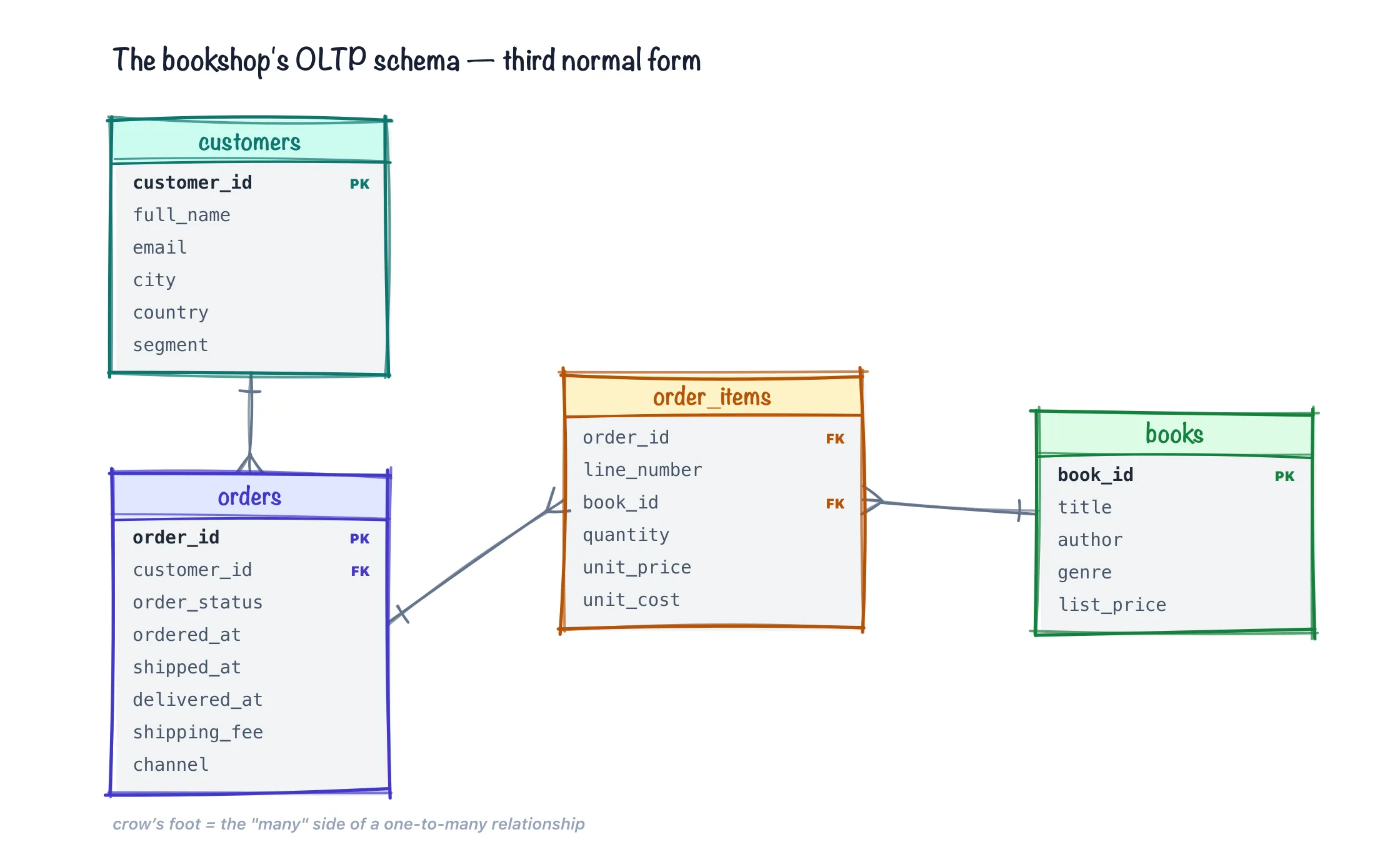
The bookshop's OLTP schema: customers, orders, order_items, and books as four normalized tables, every relationship a foreign key.

That’s the whole schema — four tables, and it’s the source we spend the rest of the series remodeling. Keep it handy; every fact and dimension we build traces back to these.

Now answer one question against it: revenue by genre by month. Here’s the query, in full, with every trap it contains:

select
    date_trunc('month', o.ordered_at)      as order_month,
    b.genre,
    sum(oi.quantity * oi.unit_price)       as revenue
from order_items as oi
join orders      as o  on oi.order_id = o.order_id
join books       as b  on oi.book_id  = b.book_id
where o.order_status != 'cancelled'
group by 1, 2
order by 1, 2

Three joins, and every line past select is tribal knowledge. Revenue is quantity * unit_price off the line — not the list_price sitting on the book, which is what half the analysts will grab first, and which disagrees with reality every time a discount was applied. Cancelled orders have to be filtered, and you have to know the status value is the string 'cancelled' and not 'CANCELED' or a code. The date lives on the order but the genre lives on the book, so you need both joins even though you’re selecting from neither table. Miss any of these and the query still runs — it just returns a confident, wrong number.

And this schema is being merciful. Four tables is the teaching version; the production version of this app normalizes genre into a genres table, author into authors, and the shipping address into addresses, because that’s what good OLTP design does. Against that schema the same six-word question looks like this:

select
    date_trunc('month', o.ordered_at)      as order_month,
    g.genre_name,
    sum(oi.quantity * oi.unit_price)       as revenue
from order_items as oi
join orders      as o  on oi.order_id    = o.order_id
join customers   as c  on o.customer_id  = c.customer_id
join addresses   as a  on c.address_id   = a.address_id   -- "by region" someday
join books       as b  on oi.book_id     = b.book_id
join genres      as g  on b.genre_id     = g.genre_id
where o.order_status != 'cancelled'
group by 1, 2

Five joins to answer a question a manager can ask in six words — and the join order matters to whoever reads it next, and the fan-out risk is real (join orders to order_items the wrong way around a distinct count and you’ll double-count silently). The schema that makes the app fast makes the analyst slow, and worse than slow: unreliable, because every analyst re-derives this query from scratch and each re-derivation is a fresh chance to get a rule wrong.

Two databases, two jobs

This isn’t a flaw in the app database. It’s a database doing the job it was built for, which is a different job than analytics.

An application database is an OLTP system — online transaction processing. It handles a firehose of small writes: someone places an order, updates an address, cancels a line. It’s normalized precisely so those writes are cheap and safe. Store each fact once and there’s no chance of two rows disagreeing about a customer’s email, and no fan-out of updates to keep in sync. Normalization is a write-side virtue.

The physical layout matches the workload. OLTP databases are row stores: all of a row’s columns sit together on disk, because the app’s unit of work is a row — fetch order 4471, update its status, commit. An index seek finds the row, one page read retrieves everything about it. That’s a few milliseconds per transaction, thousands of times a second.

Analytics is OLAP — online analytical processing — and it inverts every one of those assumptions. Almost nothing writes; everything reads. The queries are wide and aggregate: sum this, group by that, across millions of rows and years of history. Run the revenue query against a row store with 100 million order lines and you read all of every row to use three columns of it — if a row is 200 bytes, that’s on the order of 20 GB of I/O to touch maybe 2 GB of relevant data, most of an order of magnitude wasted before the query even starts thinking.

Warehouses like Snowflake are built the other way around. Storage is columnar — each column stored contiguously and compressed, so a query reads only the columns it names, and a column of repetitive values (a genre, a status) compresses brutally well. A status column holding one of five strings compresses to a fraction of its raw size; a sorted date column nearly disappears. Between column selection and compression, the physical read for that revenue query drops from tens of gigabytes to hundreds of megabytes, before any cleverness about skipping rows even enters the picture. Execution is massively parallel — the scan fans out across compute so a billion-row aggregate is a few seconds of many machines rather than minutes of one. The Snowflake foundations series covered that machinery; the point here is what it means for schema design. What’s expensive flipped. OLTP pays for wide reads and doesn’t care about joins on indexed keys, because it touches ten rows at a time. OLAP shrugs at wide reads — it only pulls the columns you name — but pays real money for joins, because a join at analytical scale means building hash tables over millions of rows and shuffling data between compute nodes. Eight normalized tables in a query is eight of those.

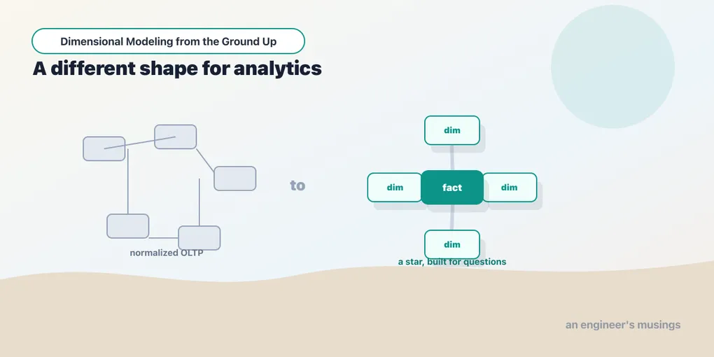
So the same data wants two different shapes. Normalized for the app that produces it, denormalized for the warehouse that questions it. Dimensional modeling is how you get the second shape — a deliberate remodel that optimizes for two audiences the OLTP schema ignores: a human who wants to ask a question without a data dictionary, and a warehouse that wants to answer it without a join marathon.

”Can’t we just use views?”

Every team meets this fork in the road, and the tempting path has three well-worn variants. They’re worth taking seriously, because each one works for about six months.

Variant one: a layer of reporting views over the OLTP schema (usually on a read replica, so the app doesn’t feel the scans). This fixes exactly one problem — analysts stop hammering production — and leaves every other one intact. A view is a saved query, not a saved result: create view revenue_by_genre still executes the five joins every time someone opens the dashboard, so you’ve moved the join marathon, not retired it. The obvious patch is to materialize the views, and now you’ve backed into building a warehouse anyway, except ad hoc: you own refresh scheduling, you own staleness monitoring, and you own the dependency ordering between views, all without any of the tooling a real transformation layer provides. And the views are welded to the app’s schema, which means every app migration is now also an analytics incident. The app team renames ordered_at to created_at in a Tuesday deploy and every downstream view breaks Wednesday morning, discovered by whoever opens the dashboard first.

Variant two: let the BI tool do the joining. Modern BI tools happily hold a join graph — point them at the normalized tables, define the relationships once, and let drag-and-drop generate the SQL. This is better than nothing and worse than it looks. The business logic — revenue means quantity * unit_price, cancelled orders don’t count — now lives inside one tool’s proprietary semantic layer, invisible to anything else. The day a second tool arrives (it always arrives), the rules get re-implemented there, and the two drift. Meanwhile there’s no place to test any of it: no assertion that order IDs are unique, no check that a status value didn’t change spelling. The logic exists, but it isn’t software — it’s configuration, in a UI, unversioned.

Variant three: just write good queries and share them. The wiki page of blessed SQL. This is the status quo the opening query described, with extra steps.

The common failure is the same in all three: the transformation logic — the joins, the filters, the business definitions — has no home. It’s re-executed per query, re-implemented per tool, or re-derived per analyst. Dimensional modeling gives it a home: the logic runs once, in a pipeline, producing real tables that are simple to query, cheap to scan, and possible to test. Views, BI joins, and shared snippets all answer “where does the query live?” The warehouse model answers the better question: “why is the query still hard?”

There’s also a capability gap no view layer can paper over: history. The OLTP database stores the current state — when a customer moves from Boston to Denver, the app updates the row, and the fact that she was a Bostonian when she placed her first forty orders is simply gone. Views over that schema inherit the amnesia. A warehouse model can choose to remember, and the machinery for that choice — slowly changing dimensions — is a chapter of its own later in the series. You can’t bolt it onto a view.

Who owns this, and what gets built first

A remodel implies a remodeler. In most teams the warehouse model is owned by analytics engineers — the role the dbt series was really about — sitting between the app teams who produce raw data and the analysts who consume the model. The boundary matters more than the title: upstream teams own the sources and are on the hook for delivering them intact and on time; the analytics engineer owns everything from the raw landing zone to the marts, including the business rules encoded along the way. When “revenue by genre” is wrong, there’s a name attached to the model that defines revenue — which is a governance upgrade over “whoever wrote that dashboard query in 2023.”

Ownership also forces the planning question: which models, for whom, in what order? Kimball’s tool for this is the bus matrix — a grid of business processes down the side, dimensions across the top, with a mark where a process needs a dimension. Even the bookshop’s toy version is clarifying:

Business process	Customer	Book	Date	Promotion
Orders placed	✓	✓	✓	✓
Inventory levels		✓	✓
Order fulfillment	✓		✓
Promotions run		✓	✓	✓

Read it column-wise and the plan falls out: Book and Date are needed by nearly every process, so they get built first and built once — every fact table that needs a calendar joins to the same dim_date, not to four departmental copies that disagree about when Q1 ends. That shared-dimension discipline is called conformance, it’s the difference between a warehouse and a pile of marts, and it gets a full treatment later in the series. For now the takeaway is that the matrix is the design deliverable that comes before any SQL: it’s how you decide what to model, and it’s one page.

The three-layer architecture

The remodel doesn’t happen in one leap from raw tables to a star. It moves through named layers, and the naming is worth being pedantic about because the whole industry has converged on roughly the same three:

Staging — one model per raw source table, cleaned and standardized but not reshaped. Rename columns into house style, cast types, apply row-level rules. No joins. This layer is the “before” photo with better manners.
Intermediate — optional, and empty until it isn’t. When a transformation is too involved to inline in a mart (a multi-step deduplication, a pivot, a windowed calculation reused by two facts), it gets its own model here rather than being pasted into two places. The bookshop’s version will arrive when we need it: turning a stream of inventory movements into end-of-day stock levels is a windowed computation that two different facts will eventually want, and it belongs in one intermediate model, not two marts.
Marts — the dimensional layer. Facts and dimensions, the tables analysts actually query. This is where the star takes shape, and it’s where the rest of this series lives.

If you’ve heard the medallion vocabulary — bronze, silver, gold — it’s the same idea wearing lakehouse clothes: bronze is the raw landing zone, silver is staging, gold is marts. dbt’s own project-structure guidance names the layers staging/, intermediate/, marts/, and that’s the convention this series follows, with one directory per layer under models/.

The rule that makes the layers mean something: business logic moves downstream, never upstream, and each rule lives in exactly one layer. Row-level cleaning (types, renames, filters that define what a valid record is) belongs in staging. Reshaping and business calculations belong in marts. A rule that lives in two layers will eventually disagree with itself.

Where we start: the “before” shape

This series remodels the bookshop from its OLTP shape into a star, one concept per post, each built in dbt on Snowflake — the setup from The Modern Data Stack. But you can’t remodel data you haven’t captured, so the first move isn’t dimensional at all: pull the raw OLTP tables into dbt, faithfully, before changing their shape.

Declare them as sources, and make the declaration earn its keep — a source definition is also where freshness expectations live:

# models/staging/_sources.yml
version: 2

sources:
  - name: raw
    database: bookshop
    schema: raw
    loaded_at_field: _loaded_at
    freshness:
      warn_after: {count: 12, period: hour}
      error_after: {count: 24, period: hour}
    tables:
      - name: orders
      - name: order_items
      - name: customers
      - name: books

The _loaded_at column is the timestamp your ingestion tool stamps on every row it lands — Fivetran, Airbyte, and a hand-rolled COPY INTO can all provide one. With it declared, dbt source freshness compares max(_loaded_at) to the clock and warns or errors per the thresholds — so “the pipeline ran but the data is stale” becomes an alert instead of a dashboard mystery. The thresholds are set per-source here and can be overridden per-table when one feed is slower than the rest. Running it looks like this:

$ dbt source freshness
12:01:11  1 of 4 START freshness of raw.orders ................ [RUN]
12:01:12  1 of 4 WARN freshness of raw.orders ................. [WARN in 0.94s]
12:01:12  2 of 4 START freshness of raw.order_items ........... [RUN]
12:01:13  2 of 4 PASS freshness of raw.order_items ............ [PASS in 0.81s]
...

A WARN on orders while order_items passes tells you something a failed dashboard never could: one feed is lagging, the others are fine, and the problem is upstream of dbt entirely. (The dbt sources post covers the full surface.)

Then give each source table a staging model: a clean restatement of a single raw table, renamed into your house style, retyped where you don’t trust the source, with the rows you never want handled explicitly.

-- models/staging/stg_orders.sql
{{ config(materialized='view') }}

with source as (
    select * from {{ source('raw', 'orders') }}
),

renamed as (
    select
        order_id,
        customer_id,
        lower(order_status)               as order_status,
        cast(ordered_at as date)          as order_date,

        -- the fulfilment milestones the accumulating snapshot needs (chapter 5).
        -- Null until they happen — which is the point.
        cast(shipped_at   as date)        as ship_date,
        cast(delivered_at as date)        as delivery_date,

        shipping_fee,

        -- the order-level flags the junk dimension collects (chapter 13)
        is_gift_wrapped,
        is_expedited,
        is_first_order,
        channel,

        cast(updated_at as timestamp_ntz) as updated_at,

        -- flag, don't filter. See below.
        (lower(order_status) = 'cancelled') as is_cancelled
    from source
)

select * from renamed

Two decisions in there are worth defending, because both are the kind you make once and live with for the life of the warehouse.

Flag cancellations; don’t filter them. The tempting line is where order_status != 'cancelled' — cancelled orders aren’t revenue, so why carry them? Because “isn’t revenue” is a question the marts should answer, not the staging layer. Filter here and a cancelled order doesn’t just leave the revenue mart, it ceases to exist: you cannot count cancellations, cannot compute a cancellation rate, and — worse — an order that gets cancelled after it was loaded silently vanishes from staging, leaving its row in the accumulating snapshot hanging open forever, waiting for a delivery that will never come. Staging’s job is to make the source usable, not to make it smaller. Carry the row, carry the flag, and let each mart decide.

The milestone dates are nullable, on purpose. ship_date and delivery_date are null for an order that hasn’t shipped. That is not missing data; it is data that says “not yet,” and chapter 5’s accumulating snapshot exists precisely to fill those in over time.

The two-CTE shape — source at the top, renamed doing the work — is the house pattern for every staging model. It looks like ceremony on a model this small, and it pays off the moment a model needs a second input or a third step: inputs are declared at the top, transformations read top-to-bottom, and every staging file in the project has the same silhouette. The casts are not optional politeness. Sources lie about types — a date arrives as a string, an amount as text with a currency symbol, and the staging layer is where those lies get caught, once, instead of in every downstream model. Same story for lower(order_status): the source has been observed emitting both 'Cancelled' and 'cancelled', so staging normalizes case before anything filters on it.

One column deserves a special mention: updated_at is carried through even though no report will ever group by it. It’s operational metadata, the timestamp the app last touched the row, and keeping it in staging is cheap insurance. When the fact tables later become incremental (rebuilding only what changed instead of everything, every run), updated_at is how a correction to an old order gets noticed. Staging models that drop it force an awkward retrofit later, so the house rule is simple: keep the source’s change-tracking columns, always, whether or not you can articulate the use yet.

Naming, briefly: dbt’s convention for staging models is stg_<source>__<entity> (double underscore), which matters when two sources both have an orders table. The bookshop has one source, so this series uses the short form — stg_orders, stg_books — but the long form is what you’d reach for at work.

Staging models are views by default, and that’s the right default: they’re a thin rename over the source, storage-free, always current. The exception is a staging model over a genuinely huge raw table that many marts read repeatedly — there, materializing as a table (or incrementally, once you’ve read the incremental models post) trades storage for not re-scanning raw on every downstream build. Start with views; promote when the warehouse bill argues for it.

And staging is where the first tests go — because a broken assumption is cheapest to catch at the boundary where the data enters:

# models/staging/_staging.yml
version: 2

models:
  - name: stg_orders
    columns:
      - name: order_id
        data_tests:
          - unique
          - not_null
      - name: status
        data_tests:
          - accepted_values:
              values: ['placed', 'paid', 'shipped', 'delivered']

The accepted_values test is quietly the most protective one in the file. The day the app team adds a 'refunded' status, this test fails on the next run — loudly, in the pipeline — instead of 'refunded' orders silently flowing into revenue because no filter knew to exclude them. Tests on staging are a contract with the source: this is what we believe about your data, checked on every build.

What staging is not

Here’s the part that matters for this series: notice what staging doesn’t do. stg_orders is still the OLTP shape — one model per source table, no joins, no facts, no dimensions, just raw.orders with better manners. That’s deliberate. Staging never joins, because the moment it does, it has opinions about shape, and shape is the marts layer’s job. Everything from the next post on is the remodel: collapsing these normalized tables into the fact and dimension tables of a star.

The one modeling decision already earning its keep is that cancelled-order filter. “Cancelled orders don’t count” was tribal knowledge scattered across every analyst’s ad-hoc query in the OLTP world; here it’s written down once, in a file, in git. It’s worth pausing on the choice, though, because a hard filter is the aggressive version of the rule. The alternative is to keep cancelled rows and expose an is_cancelled flag, letting each mart decide — which you’d want if anyone will ever ask “how many orders get cancelled?” (a real question about a real business process). The bookshop’s rule is that cancelled orders are noise, so we drop them at the door; the honest general advice is to flag by default and filter only when you’re sure the excluded rows answer no question anyone will ask. Either way, the rule lives in staging, once — that’s the point.

One assumption is hiding in these models, and it’s worth naming before it bites: every customer_id on an order is presumed to exist in customers. In real pipelines that presumption fails — an order lands before its brand-new customer record does, or a source purge orphans old keys — and a naive model either drops those orders on a join or leaves a hole where a customer should be. Dimensional modeling has a specific, slightly odd-looking answer (a designated “unknown member” row in every dimension, so no fact ever points at nothing), and it arrives in the dimensions post. File the problem for now: referential integrity between sources is a hope, not a guarantee, and the model has to be built for the days it doesn’t hold.

Final thoughts

The instinct to reuse the app’s schema for reporting is the single most expensive shortcut in analytics. It feels efficient — the data’s right there, why remodel it? — and it quietly taxes every query and every analyst for the life of the warehouse. Normalization and analytics want opposite things, and pretending otherwise doesn’t make the joins go away; it just moves them into every dashboard, every BI tool config, every analyst’s muscle memory, where they’re re-paid daily and tested never. Dimensional modeling is the decision to pay that cost once, on purpose, in a shape everyone downstream inherits for free — and the staging layer built in this post is the foundation it stands on: sources declared, freshness watched, types settled, rules written down in exactly one place.

Next: The Star Schema