Teaching a Model to See: Convolution and LeNet

Series: Practical PyTorch: Running Models — Vision — Part 1 of 5

Last post traced the Linear family — perceptron, logistic regression, the MLP that cracked XOR. Every one treats its input as a flat, unordered list of numbers. That’s fine for a row of features, but it’s the wrong shape of mind for an image, where the whole point is that pixels have neighbors. This post introduces the one new layer that fixes that — convolution — and builds up to LeNet, the first famous convolutional network. It’s the last idea you need before we open a real deep model next post.

▶ Open the companion notebook in Colab

Your MLP can already eat an image

Here’s the thing: nothing stops you from feeding an image to the MLP you built last post. An image is just a grid of numbers — a 28×28 grayscale digit is 784 of them — and if you flatten that grid into a row, a Linear will happily take it:

import torch
import torch.nn as nn

mlp = nn.Sequential(
    nn.Flatten(),            # a 28x28 image -> a row of 784 numbers
    nn.Linear(28 * 28, 100),
    nn.ReLU(),
    nn.Linear(100, 10),      # 10 digit classes
)

img = torch.rand(1, 1, 28, 28)   # one 1-channel 28x28 image
print(mlp(img).shape)            # torch.Size([1, 10]) — it runs!

It runs. People really did classify digits this way, and it sort of works. But “sort of” is the operative word, because flattening throws something precious away.

Three things go wrong

• It ignores layout. The moment you flatten, pixel (0,0) and its neighbor (0,1) become “input #1” and “input #2” — no more related, as far as the model is concerned, than two random entries in the row. Every fact about nearby pixels forming an edge, a curve, a stroke is gone. The model has to rediscover spatial structure from scratch, with no hint that the grid ever existed.
• The parameters explode. That first Linear connects every input to every hidden unit. For a small grayscale image into a modest hidden layer, that’s already enormous:

big = nn.Linear(28 * 28, 1000)
print(sum(p.numel() for p in big.parameters()))   # 785,000 parameters

785,000 weights — for one tiny grayscale image into one layer. A real color photo is millions of pixels; the math falls apart fast.

• It can’t generalize across position. Shift the digit one pixel to the right and every input value changes, so the network sees something entirely new. It has to learn the “7” all over again in its new spot. A model that has to relearn a shape everywhere it might appear is a model fighting itself.

Convolution fixes all three at once — and that’s the whole idea LeNet is built on.

Convolution: slide a small filter

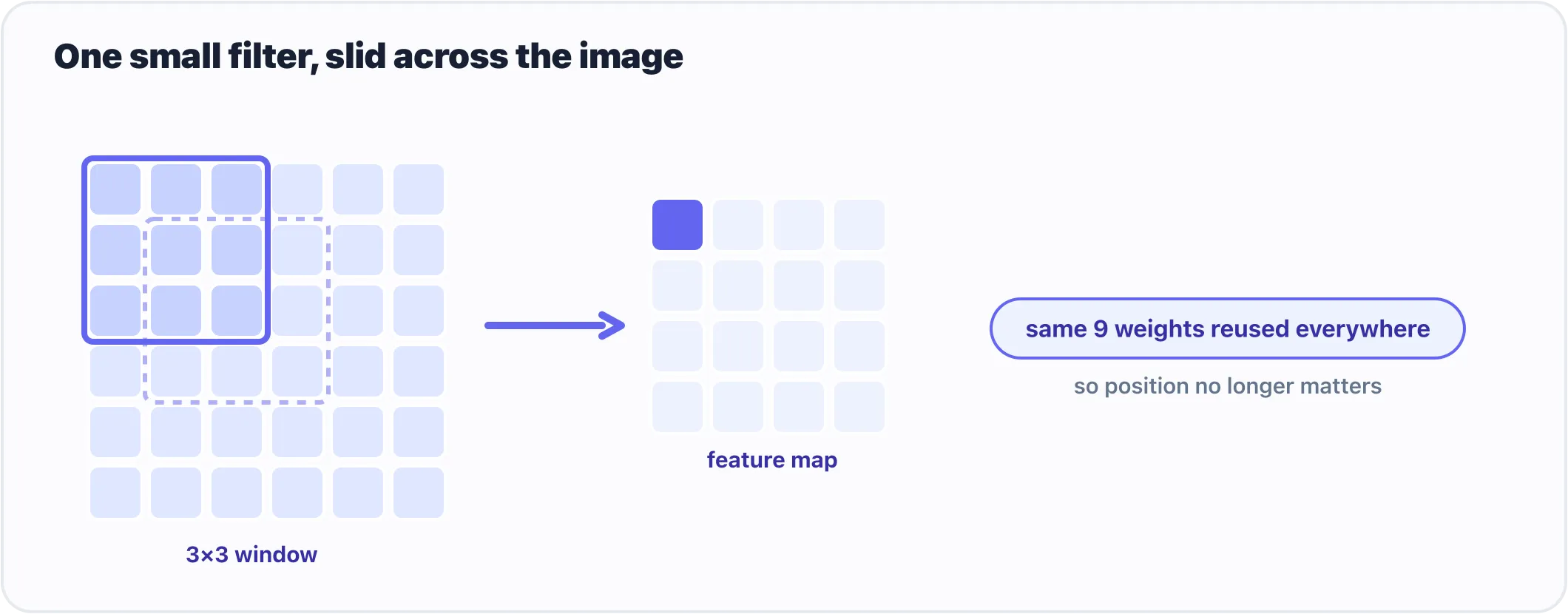
One small filter slides across the image, reusing the same weights at every position.

The new layer is nn.Conv2d, and its one-line intuition is slide a small filter over the image. Instead of wiring every pixel to every output, a convolution takes a tiny window — say 3×3 or 5×5 — and drags it across the picture, looking for one pattern (an edge, a corner, a blob of color) and reporting where it found that pattern. One filter, slid over the whole image.

Watch how that one move solves all three problems:

• It respects layout. The filter only ever looks at a pixel together with its neighbors — the little window — so spatial structure is baked in, not thrown away.
• It barely has any parameters. A 5×5 filter is 25 numbers, reused at every position. You’re not learning a separate weight per pixel; you’re learning one small pattern-detector and applying it everywhere. That’s why a convolution can scan a huge image with a handful of weights.
• It generalizes across position. Because the same filter slides everywhere, a “7” detected in the corner uses the exact same weights as a “7” in the center. Learn the pattern once, spot it anywhere.

Stack a few convolutions and the model builds up a hierarchy on its own: early layers catch edges, later ones assemble edges into shapes, and shapes into whole digits. This is the workhorse of every vision model built since — including the ResNet we’ll read next post.

Pooling and flattening

Two small supporting layers ride along with convolution in almost every CNN:

• nn.MaxPool2d — shrink the image by keeping only the strongest signal in each little patch (e.g. the largest value in every 2×2 block, halving the height and width). It throws away precise position while keeping “was the pattern here, roughly?”, which makes the model smaller and a little more robust to small shifts.
• nn.Flatten — the bridge back to the Linear world. After the convolutions and pooling have distilled the image into a small stack of feature maps, you flatten that into a row and hand it to one or two Linear layers to make the final decision. (Same Flatten as before — but now it runs on a tiny, already-digested grid, not the raw pixels.)

So a CNN is a sandwich: convolutions and pooling to see, then Linear layers to decide.

Building LeNet

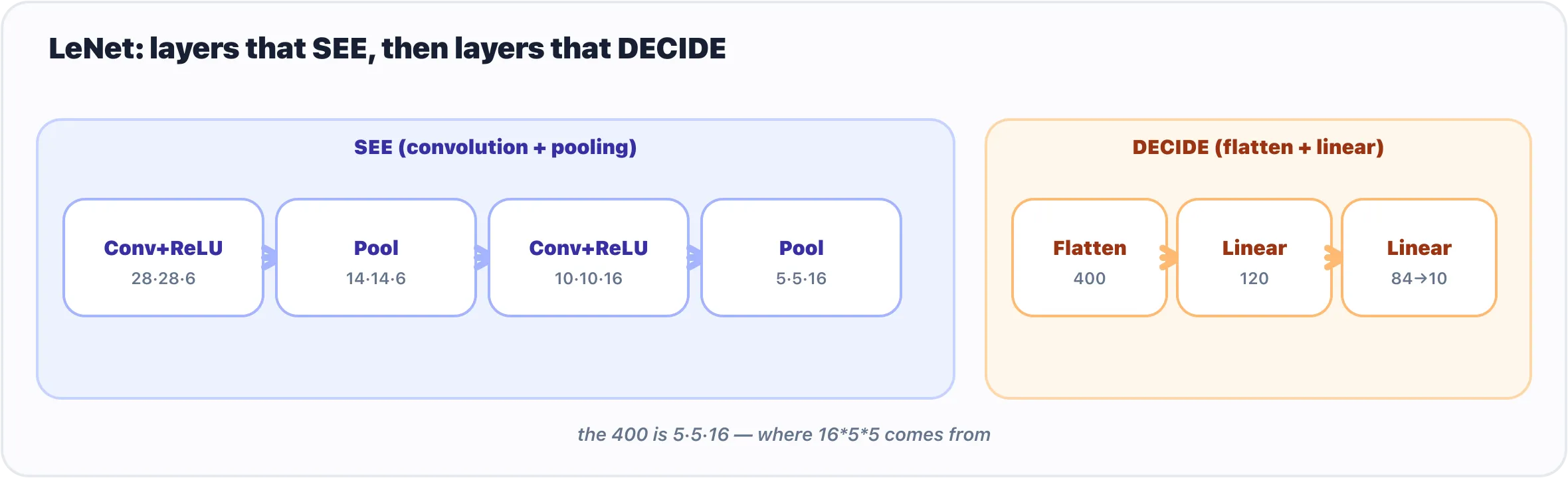
LeNet is a sandwich: convolution and pooling that see, then linear layers that decide.

Put it together and you have LeNet-5 (Yann LeCun, 1998) — the first convolutional network to do a real job, reading handwritten digits well enough to sort mail and cash checks. It’s still the same nn.Sequential you know, now with the new layers in the mix:

lenet = nn.Sequential(
    nn.Conv2d(1, 6, kernel_size=5, padding=2),  # slide 6 filters over a 1-channel image
    nn.ReLU(),
    nn.MaxPool2d(2),                            # halve the height and width
    nn.Conv2d(6, 16, kernel_size=5),
    nn.ReLU(),
    nn.MaxPool2d(2),
    nn.Flatten(),                               # grid -> a flat row, to hand to Linear
    nn.Linear(16 * 5 * 5, 120),
    nn.ReLU(),
    nn.Linear(120, 84),
    nn.ReLU(),
    nn.Linear(84, 10),                          # 10 outputs — one per digit, 0 through 9
)

total = sum(p.numel() for p in lenet.parameters())
print(f"{total:,} parameters")                  # 61,706 parameters

Read it top to bottom and it’s exactly the sandwich: two Conv2d+ReLU+MaxPool2d stages that see, a Flatten, then three Linear layers that decide, ending in 10 outputs — one per digit. And look at the count: 61,706 parameters for the whole thing, counted with the same one-liner from the build-a-model post. Compare that to the 785,000 a single flat Linear layer wanted a moment ago. Convolution didn’t just see better; it did it with a fraction of the weights.

(As in the perceptron-to-deep-net post, this is the architecture — fresh, untrained, random weights. Its shapes all line up and it runs, but it won’t recognize a digit until it’s trained on data, which is the Training Models series’ job. Here we build it to read it.)

What’s next

You’ve now met the whole toolkit a vision model is made of: Conv2d to slide filters and respect the image, MaxPool2d to shrink, Flatten and Linear to decide. LeNet stacks them a few deep and reads digits. The only thing standing between it and a modern image classifier is more — more layers, more filters, more data.

So let’s open one. ResNet-18 is exactly that: LeNet’s idea stacked far deeper, shipped with real pretrained weights and eleven million numbers inside — and you’ll find nothing in it but the layers you just met.

Next: Reading a Real One: ResNet Up Close, where we open a famous deep network and read it like the spec sheet it is.

---

Target keyword(s): pytorch convolution, nn.Conv2d explained, what is a CNN, LeNet pytorch, why convolution for images.