Teaching a Model to Read: Attention and the Transformer

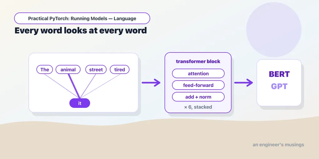
Series: Practical PyTorch: Running Models — Language — Part 2 of 9

You can now turn a sentence into a row of word-vectors (Part 1), but a pile of vectors isn’t reading. Those vectors have to combine, each word shaped by the others, and none of the layers you’ve built so far can do that. A grid-of-pixels assumption ran through the whole vision arc — convolution, ResNet — where what matters is local, a patch at a time. Language breaks that assumption completely. A sentence is a sequence, the meaning of a word can hinge on another word twenty positions away, and “the bank raised rates” and “the river bank” turn on context, not on neighboring letters. This post introduces the one idea that handles all of that — attention — and builds up to the transformer, the architecture behind essentially every language model you’ve used. Math-free, no training, just the shape of the thing.

▶ Open the companion notebook in Colab

Why a Linear or a Conv can’t read

Try to feed a sentence to the tools you already have and you hit a wall, the same way an MLP hit a wall on images.

• A Linear layer has no sense of order. Flatten “dog bites man” into a row of numbers and it’s the same bag of words as “man bites dog” — yet the meaning flipped. Word order carries the message, and a fully-connected layer treats its inputs as an unordered list, exactly the flaw that sank the MLP on images in the convolution post.
• A Conv2d only looks locally. Convolution’s whole trick is the small window: it sees a pixel with its immediate neighbors. That’s perfect for edges and strokes, and useless for “this pronoun refers to that noun at the start of the paragraph.” Language is full of long-range ties that no small sliding window can reach.
• Reading one word at a time is slow and forgetful. The older fix, the recurrent network (RNN), walked the sentence left to right, carrying a running memory. It worked, but it processed words strictly in sequence (so it couldn’t use a modern GPU’s parallelism well) and its memory faded over long distances: the words at the start were a rumor by the end.

What you’d really want is a layer where every word can look directly at every other word and decide, for itself, which ones matter. That’s attention.

Attention: every word looks at every other

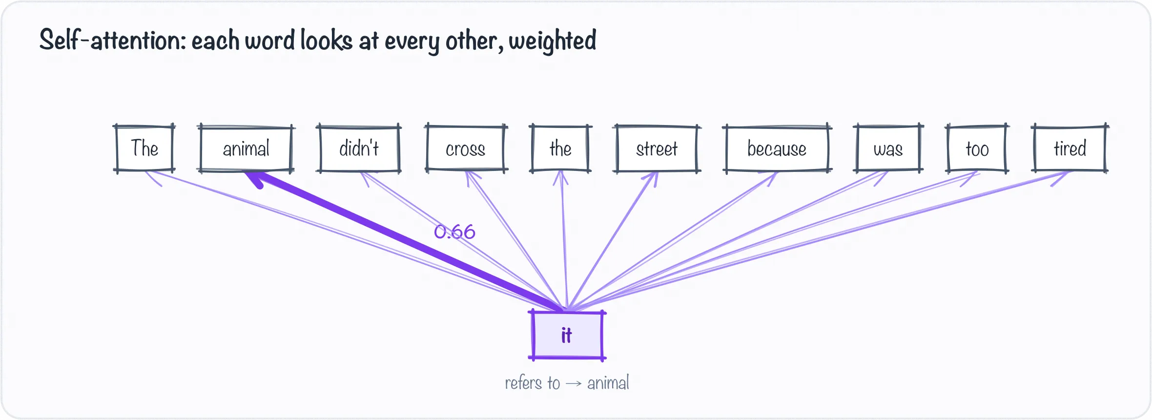
Self-attention lets every word weigh every other — here “it” leans almost entirely on “animal.”

Here’s the whole intuition in one sentence: attention lets each word gather information from all the other words, weighted by how relevant each one is.

Take “The animal didn’t cross the street because it was too tired.” What does “it” refer to? You know instantly: the animal, not the street. Attention is the mechanism that lets the model figure out the same thing. When the model processes “it,” attention lets that position look at every other word and assign each a weight — a high weight on “animal,” a low weight on “street” — then build “it“‘s representation as a blend of the words it decided were relevant. Every word does this, for every other word, at the same time.

That “for every other word” is the key difference from a sliding window. Attention isn’t local. The word at position 2 can attend just as easily to position 200 as to position 3: distance costs it nothing. The long-range tie that defeated convolution is the thing attention does first.

When a layer does this with the sentence looking at itself — every word attending to every other word in the same sequence — it’s called self-attention, and it’s the engine of the whole architecture.

The transformer block: attention plus a little thinking

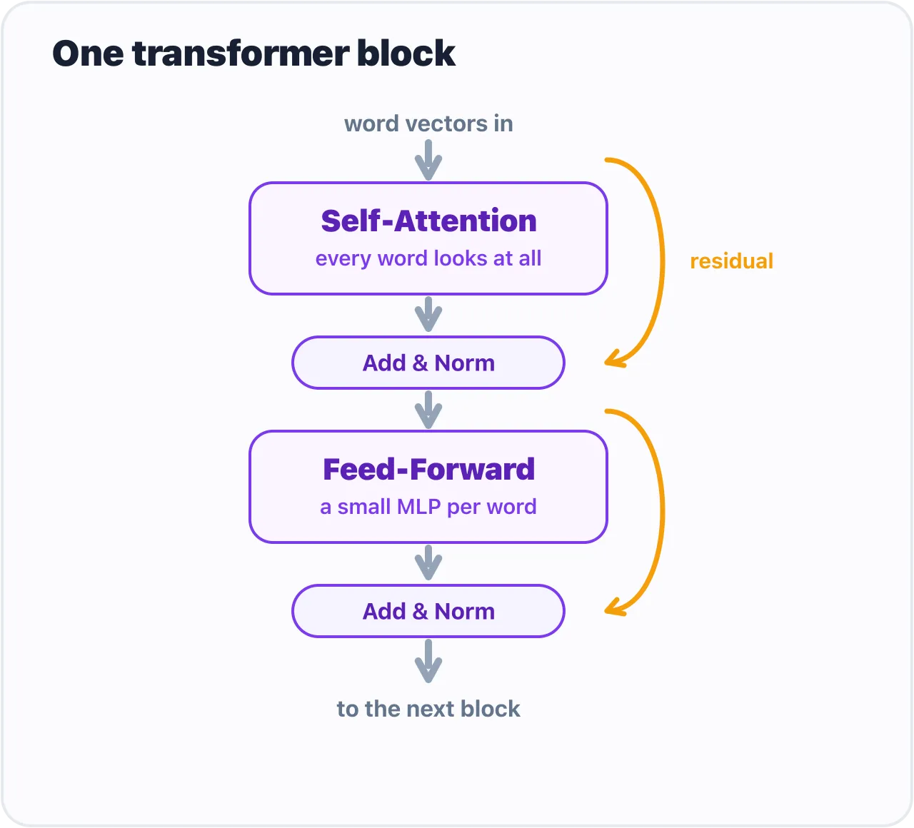
One transformer block: self-attention, then a feed-forward MLP, each wrapped by a residual and a norm.

Attention on its own gathers context, but it doesn’t do much with it. So a transformer pairs it with a small ordinary network and stacks the pair. One transformer block is just two steps:

1. Self-attention — every word gathers relevant context from the rest of the sentence.
2. A feed-forward network — a small MLP (two Linear layers with a nonlinearity between them, exactly the kind you built back in Foundations) that processes each position a little further.

Two supporting pieces ride along, and you can read past them the way you read past BatchNorm in ResNet: a residual connection (add the input back after each step, so signal and gradients flow cleanly through a deep stack) and layer normalization (keep the numbers in a steady range). Attention, feed-forward, add, normalize — that’s the block.

A “transformer” is just a tall stack of these identical blocks. The famous models differ mostly in how many they stack and which way they face (more on that below), not in what’s inside each one.

Building a block you can print

Here’s the part that should feel familiar from the convolution post: this isn’t a mysterious new object, it’s an nn.Module you can build and print. PyTorch ships a ready-made transformer block, nn.TransformerEncoderLayer.

Start small enough to connect to the twelve-word toy from Part 1. Its embedding turns the sentence into vectors; size a block to match those, and push them straight through:

import torch
import torch.nn as nn

# the lookup from Part 1: a 12-word vocab, 4 numbers per word
embed = nn.Embedding(12, 4)
ids = torch.tensor([[0, 2, 4, 6, 0, 7]])   # "the cat sat on the mat", batched
emb = embed(ids)                           # [1, 6, 4] — six word-vectors

block = nn.TransformerEncoderLayer(
    d_model=4,              # match the embedding width
    nhead=2,                # heads split d_model into equal parts, so it must divide 4 (not 8)
    dim_feedforward=8,      # the little MLP's hidden size
    batch_first=True,
)
out = block(emb)
print(out.shape)               # torch.Size([1, 6, 4])

total = sum(p.numel() for p in block.parameters())
print(f"{total:,} parameters")   # 172 parameters

Same shape in, same shape out: six word-vectors go in, six come back. Each one has now been blended with the others by attention. Rewriting every word’s vector using the rest of the sentence is the block’s whole job, and it does that without changing how many words there are or how wide they sit.

Now scale it to the sizes a real model uses, and print the block to read its parts:

block = nn.TransformerEncoderLayer(
    d_model=128,            # the size of each word's vector
    nhead=8,                # run attention 8 ways in parallel ("heads")
    dim_feedforward=512,    # the hidden size of the little MLP
    batch_first=True,
)
print(block)

The printout is the block laid bare — and every line is something you’ve now met:

TransformerEncoderLayer(
  (self_attn): MultiheadAttention(...)        # every word looks at every word
  (linear1): Linear(in_features=128, out_features=512, bias=True)   # the feed-forward MLP
  (linear2): Linear(in_features=512, out_features=128, bias=True)
  (norm1): LayerNorm((128,), ...)             # keep the numbers steady
  (norm2): LayerNorm((128,), ...)
  ...
)

There it is: self_attn (the new idea), two Linear layers (the feed-forward network), and a couple of LayerNorms (the supporting cast). Notice what’s not in there: no embedding. The block works on vectors, so the word-to-vector lookup (the nn.Embedding you ran above) happens once up front, not inside each block. Count its parameters with the same one-liner from the build-a-model post:

total = sum(p.numel() for p in block.parameters())
print(f"{total:,} parameters")   # 198,272 parameters

It’s the same block and the same recipe, only wider: widen d_model from 4 to 128 and the count climbs from 172 to about two hundred thousand, all of it random and untrained here, just like the LeNet you built in the vision arc. Stack a handful of these and give them real weights and you have a working language model. That stacking is exactly what we’ll open up next post.

nhead=8, briefly. Attention runs several times in parallel — eight “heads” here — each free to focus on a different kind of relationship (one head might track grammatical subjects, another nearby words). You don’t need the details in the Running Models series; just know that “multi-head” means “several attentions at once,” and the results are combined.

Encoder, decoder, and the models you’ve heard of

Transformers come in two flavors, and the difference is just what each word is allowed to look at:

• Encoders let every word see the whole sentence, both directions. Great for understanding a fixed piece of text: classification, search, embeddings. BERT is the famous one, and DistilBERT, which we’ll read next post, is its compact cousin.
• Decoders let each word see only the words before it, never ahead. That’s what you need to generate text one word at a time, which is why the GPT family (and the chatbots built on it) are decoders.

Same block in both cases. The whole zoo of language models is this one idea — attention, wrapped in a block, stacked deep — pointed at different jobs.

What’s next

You’ve added a third branch to the family tree. The Linear family learned to weigh features (Foundations), convolution learned to see images (Vision), and now attention has learned to read sequences — every word free to consult every other. A transformer is just that block, stacked.

So let’s open a real one. DistilBERT is a genuine, pretrained transformer with about sixty-six million numbers inside, and when we print it you’ll find nothing but the embeddings, attention, feed-forward layers, and norms you just met, repeated six times over.

Next: Reading a Real Transformer: DistilBERT Up Close, where we open a famous language model and read it like the spec sheet it is.

---

Target keyword(s): what is a transformer, self-attention explained, attention mechanism beginner, transformer architecture pytorch.