Tensors: The One Data Structure You Actually Have to Like

Series: Practical PyTorch: Running Models — Foundations — Part 2 of 7

Last post promised that tensors are the one part of PyTorch you genuinely need to be comfortable with. This is where we make good on that — and it’s friendlier than it sounds. A tensor is an array of numbers — a spreadsheet, if you like — that happens to be able to live on a GPU. That’s the whole idea. Everything a model takes in, passes around inside itself, and hands back is a tensor. Get easy with this one structure and the rest of the series is mostly knowing which buttons to press.

This post is about making and manipulating tensors — building them, looking inside them, reshaping them, doing math on them. The other superpower, moving them onto a GPU and trading them with the rest of Python, gets its own post right after this one.

Open the companion notebook and run along — every snippet below is in there:

▶ Open the companion notebook in Colab

Making a tensor

The most direct way is to hand torch.tensor a Python list:

import torch

x = torch.tensor([[1, 2, 3],
                  [4, 5, 6]])
print(x)

A flat list gives you a 1-D tensor (a row of numbers); a list of lists gives you a 2-D tensor (a grid, like a spreadsheet); nest one more level and you get 3-D, and so on. The number of nesting levels is the number of dimensions, and that’s the only piece of vocabulary you have to keep.

Most of the time, though, you don’t type numbers out by hand. You ask PyTorch to build a tensor of a given shape and fill it for you:

torch.zeros(2, 3)     # a 2x3 grid of zeros
torch.ones(2, 3)      # a 2x3 grid of ones
torch.full((2, 3), 7) # a 2x3 grid, every cell a 7
torch.arange(0, 10)   # 0, 1, 2, ... 9 — like Python's range()
torch.rand(2, 3)      # a 2x3 grid of random numbers between 0 and 1

The arguments (2, 3) are the shape: 2 rows, 3 columns. These show up constantly; rand in particular is how you fake some input data when you just want to see whether code runs before you’ve got the real thing.

One more habit worth picking up early — building a new tensor shaped like one you already have, so you don’t have to retype the dimensions:

x = torch.rand(2, 3)
torch.zeros_like(x)   # a 2x3 grid of zeros, matching x's shape

Shape, dtype, device — the three questions to ask any tensor

When a tensor confuses you, three attributes answer almost every question. Get in the habit of printing them:

x = torch.rand(2, 3)

print(x.shape)    # torch.Size([2, 3]) — how big, in each dimension
print(x.dtype)    # torch.float32     — what kind of number
print(x.device)   # cpu               — where it physically lives

• .shape is the size along each dimension. [2, 3] means 2 rows and 3 columns. When something breaks in PyTorch, the cause is usually a shape that isn’t what you assumed — so this is the first thing to check, always.
• .dtype is the kind of number: float32 (decimals) or int64 (whole numbers) most often. A list of whole numbers gives you an integer tensor; add a single decimal point and you get a float tensor. Models almost always want floats.
• .device is where the data lives: cpu to start, cuda once you move it to a GPU. That move is the whole subject of the next post; for now, just know this is the attribute that tells you.

Indexing and slicing

If you’ve used NumPy or even plain Python lists, this part is muscle memory. Square brackets pull out pieces:

x = torch.tensor([[1, 2, 3],
                  [4, 5, 6]])

print(x[0])        # first row:    tensor([1, 2, 3])
print(x[0, 1])     # row 0, col 1: tensor(2)
print(x[:, 0])     # every row, first column: tensor([1, 4])
print(x[-1])       # last row:     tensor([4, 5, 6])

Rows are counted from zero, the comma separates dimensions, a bare : means “all of this dimension,” and a negative index counts from the end. That’s the entire grammar.

Slicing pulls out ranges with the same start:stop notation Python lists use (the stop is excluded):

y = torch.arange(10)   # tensor([0, 1, 2, 3, 4, 5, 6, 7, 8, 9])

print(y[2:5])          # tensor([2, 3, 4])
print(y[:3])           # tensor([0, 1, 2])  — from the start
print(y[7:])           # tensor([7, 8, 9])  — to the end

And you can assign through an index or slice to change values in place:

x[0, 0] = 99           # one cell
x[:, 1] = 0            # a whole column at once

That second line sets every value in column 1 to zero in a single stroke — no loop. Writing to a slice is one of the quiet conveniences you’ll reach for all the time.

Reshaping

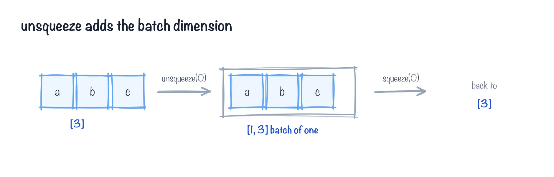
unsqueeze(0) wraps a [3] vector into a [1, 3] batch of one; squeeze(0) undoes it.

Reshaping rearranges the same numbers into a different grid without changing them. A tensor of 6 numbers can be 2×3, or 3×2, or a flat row of 6, whichever you want:

x = torch.arange(6)        # tensor([0, 1, 2, 3, 4, 5]), shape [6]
y = x.reshape(3, 2)        # same six numbers, now 3 rows of 2
print(y)

The numbers and their order never change; only the box you’re pouring them into does. You’ll see .view(...) used for the same job — it’s a faster variant that works when the data is laid out contiguously in memory. When in doubt, reach for .reshape; it always works and figures out the rest.

A handy trick: pass -1 for a dimension and PyTorch computes it for you. x.reshape(2, -1) says “2 rows, and you work out the columns.” Saves you the arithmetic.

Two close cousins of reshaping come up so often they’re worth meeting now — unsqueeze adds a dimension of size 1, and squeeze removes one:

v = torch.tensor([1, 2, 3])    # shape [3]
b = v.unsqueeze(0)             # shape [1, 3] — wrapped in a "batch of one"
print(b.shape)

print(b.squeeze().shape)       # back to [3]

That unsqueeze(0) is not busywork: models almost always expect a batch of inputs, so you routinely take a single example of shape [3] and add a leading 1 to make it [1, 3]. It’s the most common shape fix you’ll make, and you’ll see exactly why a few posts from now.

Doing things with tensors

Arithmetic on tensors happens elementwise — the operation runs on each number in turn, and you get a tensor of the same shape back:

a = torch.tensor([1, 2, 3])
b = torch.tensor([10, 20, 30])

print(a + b)   # tensor([11, 22, 33])
print(a * 2)   # tensor([2, 4, 6])
print(a * b)   # tensor([10, 40, 90]) — pairs multiplied, not "matrix math"

Note that a * b multiplies matching positions — it is not the matrix multiplication you may dimly remember from school.

That other kind — matrix multiplication — has its own operator, @:

m = torch.tensor([[1, 2],
                  [3, 4]])
n = torch.tensor([[5, 6],
                  [7, 8]])
print(m @ n)

Here’s all the intuition you need: @ is the core operation a neural network repeats over and over — it’s how a layer combines its inputs to produce outputs. You’ll see @ everywhere inside models. You do not need to be able to compute it by hand or prove anything about it; you need to recognize it and know it’s the “real” matrix multiply, as opposed to the elementwise *.

Summing things up: reductions

Often you want to boil a whole tensor down to one number, or one number per row. Those are reductions, and the common ones read exactly like what they do:

g = torch.tensor([[1.0, 2.0, 3.0],
                  [4.0, 5.0, 6.0]])

print(g.sum())    # tensor(21.) — every number added up
print(g.mean())   # tensor(3.5) — the average
print(g.max())    # tensor(6.)  — the biggest

By default a reduction collapses the entire tensor to a single value. But you can aim it along one dimension with dim= — handy when each row is a separate example and you want a per-row answer:

print(g.sum(dim=1))   # tensor([6., 15.]) — one sum per row
print(g.max(dim=0))   # the biggest in each column

dim=1 means “collapse the columns, leave the rows,” and dim=0 is the reverse. The result there, tensor(21.) or tensor(3.5), is still a tensor — just one holding a single number. When you want it as a plain Python float to print or compare, there’s a small .item() move for that, which we’ll meet in the next post alongside the rest of tensors-talking-to-the-outside-world.

A gentle word on broadcasting

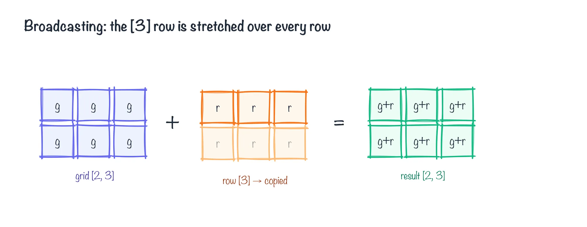
PyTorch copies the [3] row across every row of the grid — no loop required.

Sometimes you combine tensors of different shapes and it just works. PyTorch quietly stretches the smaller one to fit:

grid = torch.ones(2, 3)        # 2x3 of ones
row  = torch.tensor([1, 2, 3]) # a single row of 3

print(grid + row)
# tensor([[2, 3, 4],
#         [2, 3, 4]])

The single row got added to every row of the grid. That convenience is called broadcasting, and it’s why you often see a small thing combined with a big thing without any loops. You don’t have to memorize the rules — recognizing that PyTorch sometimes resizes things to match is enough to keep it from surprising you.

Gotchas

A few friendly trip-wires that catch nearly everyone at least once:

• Shape mismatches are the #1 error. “size mismatch” or “shapes cannot be multiplied” almost always means a tensor wasn’t the shape you pictured. Print .shape on both sides before you blame the math.
• * is not @. * multiplies matching positions; @ is matrix multiplication. Mixing them up gives you wrong numbers, not an error — the sneakiest kind of bug.
• Integer vs. float surprises. torch.tensor([1, 2, 3]) is an integer tensor; many model operations (and .mean()!) expect floats and will complain. Add a decimal point ([1.0, 2.0, 3.0]) or call .float() to convert.
• Reshaping needs the numbers to add up. You can reshape 6 numbers into 2×3 or 3×2, but not 4×2 — there aren’t eight of them. PyTorch will tell you so, loudly.
• In-place vs. a copy. A trailing underscore means “modify me in place” — x.add_(1) changes x, while x.add(1) (or x + 1) returns a new tensor and leaves x alone. When a value mysteriously changes underneath you, look for that underscore.

What’s next

That’s the data structure the entire series runs on. You can now make a tensor, ask it its shape, index and slice it, reshape it, and do arithmetic and reductions on it — which is genuinely most of what “handling data in PyTorch” means day to day. None of it required a single derivative.

There’s one more thing tensors do that we’ve kept teasing: they can leave the CPU for a GPU, and they can hand their numbers back to ordinary Python and NumPy. That’s the next post.

Next: Tensors on the Move: GPUs, NumPy, and Back, where your tensors learn to change devices and talk to the rest of your code.

---

Target keyword(s): pytorch tensors, pytorch tensors for beginners, pytorch tensor shape, pytorch reshape.