Audio Is a Tensor Too: Waveforms, Sample Rate, and Spectrograms
A beginner-friendly intro to audio in PyTorch — load a waveform with torchaudio, read its shape and sample rate, and turn it into a mel spectrogram, the image a model actually sees.
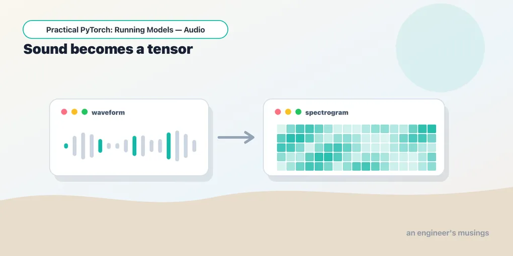
Series: Practical PyTorch: Running Models — Audio — Part 1 of 8
In the Running Models series you ran models that read and models that see — a classifier that looked at a photo and named the dog, a pipeline that read a sentence and called it positive. Sound is the third sense, and it’s the one this series is about. But here’s the thing nobody tells you at the start: a model never hears anything. It can’t. What reaches the model is a tensor of numbers, same as a sentence or a photo, and once you see which numbers, everything that follows — text-to-speech, neural codecs, generating music from a text prompt — stops feeling like sorcery and starts feeling like the work you already know.
Open the companion notebook in ColabThis whole series lives in Colab, runs pretrained models, and stays away from calculus — exactly like the Running Models series, just pointed at sound. Over the next seven posts you’ll make a model talk (text-to-speech), compare a few voices and their trade-offs, build a narrator that reads an article aloud, see how audio gets chopped into tokens by a neural codec, generate music from a typed prompt with MusicGen, learn to steer that generation, and finish by scoring your own scene. All of it rests on the one idea in this post: audio is a tensor, and it has two faces.
Sound, as a row of numbers
A microphone measures air pressure many thousands of times a second. Each measurement is a single number — how far the speaker cone (or your eardrum) is pushed at that instant. String those numbers together in time and you have a waveform: a long 1-D list of amplitudes. That’s the raw signal, and it’s the first face of the tensor.
Let’s load a real one. torchaudio ships with the tools to read audio files into tensors, and soundfile is the backend that decodes the WAV. Install both once per session:
!pip install -q torchaudio soundfileNow grab a short speech clip — torchaudio hosts a few tutorial assets you can pull down directly, so we don’t have to upload anything:
import torchaudio

# a short speech clip bundled with torchaudio's tutorial assets
path = torchaudio.utils.download_asset(
    "tutorial-assets/Lab41-SRI-VOiCES-src-sp0307-ch127535-sg0042.wav"
)
waveform, sample_rate = torchaudio.load(path)

print(waveform.shape)                          # torch.Size([1, 54400]) -> [channels, samples]
print("sample rate:", sample_rate)             # 16000
print("duration (s):", waveform.shape[1] / sample_rate)
Three numbers carry the whole picture, so let’s read them slowly.
- The shape is
[channels, samples]. This clip is mono, so one channel; the54400is how many individual amplitude readings make up the sound. Note the order: channels come first, like the color channels in an image, except here the data underneath is 1-D in time instead of a 2-D grid of pixels. - The sample rate is how many of those readings happen per second —
16000means 16,000 samples a second, written 16 kHz. It’s not metadata you can ignore; it’s the clock that gives the numbers their meaning. - Duration falls right out: samples divided by rate.
54400 / 16000is about 3.4 seconds. That’s the entire relationship between the two numbers and real time.
One more fact about the values themselves: a float waveform sits in roughly the range [-1, 1], where 0 is silence and the extremes are the loudest the signal goes. Keep that range in your head — it’s the difference between audio that plays and audio that clips.
Hear it, then see it
Because we’re in a notebook, we can actually play the tensor back. IPython.display.Audio takes a NumPy array and a rate and gives you a little player widget:
from IPython.display import Audio
Audio(waveform.numpy(), rate=sample_rate)
The rate= argument matters as much as the samples — hand the same array a different rate and it plays back too fast or too slow, chipmunk or molasses. The numbers don’t carry their own clock; you do.
Mono was easy; most music you’ll meet is stereo, with two channels (left and right) for a sense of space. Models, though, usually want a single channel. The simplest honest way to collapse stereo to mono is to average the channels:
mono = waveform.mean(dim=0, keepdim=True) # [1, samples]dim=0 is the channel dimension, so this averages left and right into one. keepdim=True keeps the result shaped [1, samples] rather than dropping to a bare 1-D tensor — which keeps that channels-first convention intact so the next step doesn’t trip on a missing dimension. (Our clip is already mono, so this is a no-op here, but it’s the line you’ll reach for the moment you load a stereo file.)
Now the picture. A waveform is just numbers over time, so the most direct plot is amplitude on the y-axis, sample index on the x-axis:
import matplotlib.pyplot as plt
plt.figure(figsize=(10, 2))
plt.plot(waveform[0].numpy())
plt.title("waveform: amplitude over time")
plt.show()
You’ll see a jagged band that swells where the speaker is talking and flattens toward silence. That’s the literal shape of the sound — every wiggle is the air pushing on the microphone. It’s honest, but it’s also a hard thing for a model to read directly: a few seconds is tens of thousands of samples, and the meaning (which words, which notes) is smeared across all of them. We need a better view.
Sample rate is part of the data
Before the better view, one detour that will save you a debugging afternoon. The sample rate isn’t a setting on the side — it’s woven into what the numbers mean, and a model trained at one rate expects audio at exactly that rate. To change it, you resample, and torchaudio has a transform for it:
resampler = torchaudio.transforms.Resample(orig_freq=sample_rate, new_freq=8000)
downsampled = resampler(waveform)
print(downsampled.shape)                        # fewer samples at 8 kHz
We’ve gone from 16 kHz to 8 kHz, so the same 3.4 seconds is now described by half as many samples. The sound covers the same span of time — it just carries less detail, the way a smaller image of the same scene has fewer pixels. The reason this matters in practice: if you ever feed 44.1 kHz audio (CD quality) to a model that expects 16 kHz without resampling first, the model reads your samples on the wrong clock and hands you confident garbage. Resample to match. Every time.
The spectrogram — audio’s image view
Here’s the second face of the tensor, and it’s the one that makes audio click for people who came in through vision. Instead of plotting amplitude over time, we plot how much of each frequency is present, over time. Low rumble at the bottom, high hiss at the top, the x-axis still time. That 2-D grid is a spectrogram, and a mel spectrogram is the version weighted to match how human hearing spaces out pitches.
torchaudio computes it with another transform:
mel = torchaudio.transforms.MelSpectrogram(sample_rate=sample_rate, n_mels=64)
spec = mel(waveform)                            # [channels, n_mels, time]
print(spec.shape)                               # torch.Size([1, 64, 273])
Look at that shape: [1, 64, 273]. One channel, 64 frequency bands (that’s our n_mels), 273 time steps. Squint and it’s the shape of an image — one channel deep, 64 tall, 273 wide. Let’s draw it as exactly that:
plt.figure(figsize=(10, 3))
plt.imshow(spec[0].log2().clamp(min=-10), origin="lower", aspect="auto")
plt.title("mel spectrogram: frequency (y) over time (x)")
plt.show()
(The log2() compresses the huge range of loudness so the quiet detail is visible, and clamp(min=-10) floors the silent parts so they don’t blow out the contrast — cosmetic, but it makes the picture readable.) What comes out looks like a heatmap: bright ridges where energy concentrates, the bands shifting as the speaker moves through vowels and consonants. You’re now seeing the speech.
And this is the bridge. A spectrogram is a 2-D grid of numbers — which is to say, an image. So a model that classifies sounds can literally be a vision model looking at spectrograms; many “audio” models are transformers or CNNs eating these pictures, not anything that processes raw waveforms at all. The convolution-over-pixels and attention-over-patches machinery from the Vision series carries straight over. You didn’t leave the world of images. You found a new way into it.
Gotchas
The handful of things that bite everyone once.
- Sample rate must match the model. Feed 44.1 kHz audio to a 16 kHz model and you get nonsense, no error to warn you. Resample with
torchaudio.transforms.Resamplefirst, every time — this is the single most common audio bug. - Shape is
[channels, time], not[time, channels]. Channels come first, the torchaudio convention (and the image convention). If a shape error looks impossible, check you haven’t got the axes flipped. - A float waveform lives in ~[-1, 1]. Load audio as integers by accident and the values jump into the thousands — which plays back as an ear-splitting surprise. When in doubt, print
waveform.min()andwaveform.max()before you hit play. - A spectrogram is lossy. It’s derived from the waveform and throws away phase (the fine timing information), so you can’t perfectly reconstruct the original sound from it. It’s a view built for models to read, not a replacement for the signal. We’ll come back to this exact limit when we generate audio later in the series.
Final thoughts
The reason this series can stay math-free is the reason this post comes first: every audio model you’ll run reduces to moving tensors around, and you already know how to do that. A waveform is a 1-D tensor of amplitudes on a clock called the sample rate; a spectrogram is a 2-D tensor that turns that signal into an image. Generating speech will mean producing one of those tensors; generating music will mean the same, with a fancier model in the middle. Hold onto the two faces, and the next seven posts are just variations on a tensor you can already read.
Next: Part 2 — Make a Model Talk: Your First Text-to-Speech Run — point a pretrained model at a sentence and get a voice back.
Target keyword(s): audio tensor pytorch, torchaudio spectrogram, waveform sample rate.
Comments