Forty-Two Percent in One Partition
A day-partitioned orders table diagnosed from its own metadata, asked the questions it was not built for, and redesigned two ways. Bucketing fixed the customer queries and taxed every day query; z-ordering did nothing at all, for a reason worth knowing.
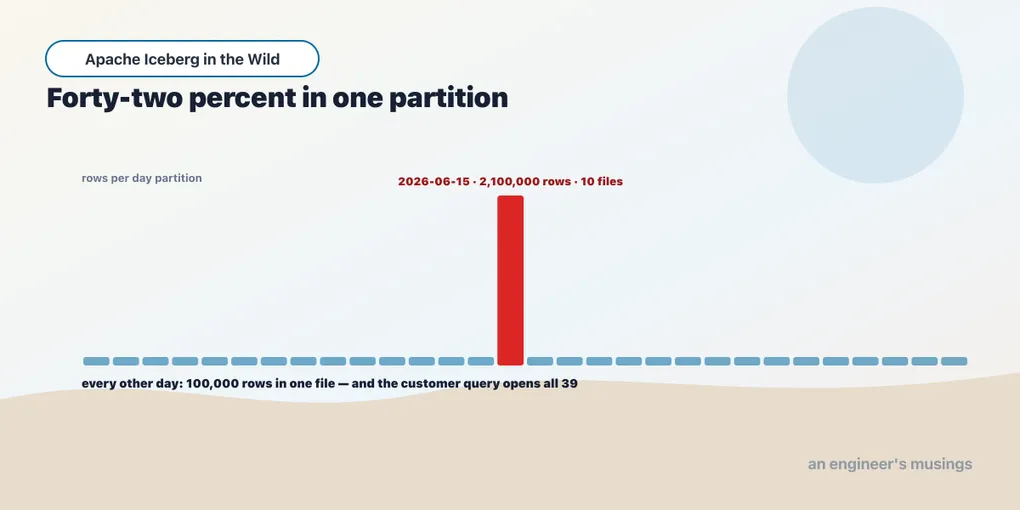
Five million orders, partitioned by day, written by a pipeline in ten batches. Two queries from the partitions and files metadata tables, nothing else, say everything that is wrong with it.
  partitions, by rows:
     2026-06-15  rows 2,100,000  files  10     4.79 MB
     2026-06-01  rows   100,000  files   1     0.15 MB
     2026-06-04  rows   100,000  files   1     0.15 MB
  30 partitions, 5,000,000 rows, 39 files; the top partition holds 42% of rows in 26% of files
  files: 39 total, min 157 KB, median 177 KB, max 0.63 MB, 39 under 1 MB (100%)
One day holds forty-two percent of the table — because there was a sale. Every file is under a megabyte, because the pipeline wrote ten batches and each batch cut a file per day. And the queries the table now gets are not the ones it was partitioned for. Three business customers hold a third of all orders between them. The questions have moved from “what did we sell on Tuesday” to “what did this customer buy”.
  sale day revenue         GETs   30  bytes    1.9 MB
  quiet day revenue        GETs    3  bytes    0.0 MB
  one retail customer      GETs   90  bytes    3.9 MB
  one B2B customer         GETs   28  bytes    1.8 MB
The day queries prune exactly as Book 1’s chapter 8 promised. The customer queries open every file because the partition spec has no customer field. The workload has changed while the layout still serves the old day-based questions. Metadata can expose the uneven partitions and small files; the query log tells us whether they still suit the workload. The two redesigns below address that mismatch — with very different costs.
What partitioning promises, and what skew is
A partition spec is a promise about predicates. It says: the queries on this table will filter on this expression often enough that laying the files out by it will pay for itself every time. Hidden partitioning, Book 1’s chapter 8, is what makes the promise cheap to keep. The transform is stored in the spec, and the reader applies it to an ordinary predicate on the source column. The promise still has to be true.
Skew is the promise going wrong in one of two ways.
Value skew is one partition holding far more rows than the others. The sale day is forty-two percent of the table. A day query on it opens ten files and reads two million rows; a day query on any other day opens one file. Every job that runs per partition, compaction included, has one task that takes twenty times longer than the rest.
Predicate skew is the queries filtering on something the spec does not cover. The customer queries are predicate skew: the spec cannot prune them, so every one is a full scan whatever the layout does inside partitions. This is the one that arrives silently — because it is a change in the workload rather than in the data.
Both are visible from metadata, and the SQL that sees them is this chapter’s artifact. It runs against any Iceberg table from any engine that exposes the metadata tables, reads no data, and takes milliseconds.
-- rows, files and bytes per partition: value skew, and the small-file ratio per partition
SELECT partition, record_count, file_count,
       ROUND(total_data_file_size_in_bytes / 1048576.0, 2) AS mb,
       ROUND(total_data_file_size_in_bytes / file_count / 1048576.0, 2) AS mb_per_file
FROM   ice.stage10.orders.partitions
ORDER  BY record_count DESC;

-- the file-size distribution: how much of the table is small files
SELECT count(*)                                                        AS files,
       ROUND(percentile_approx(file_size_in_bytes, 0.5) / 1024.0)     AS p50_kb,
       ROUND(max(file_size_in_bytes) / 1048576.0, 2)                  AS max_mb,
       sum(CASE WHEN file_size_in_bytes < 33554432 THEN 1 ELSE 0 END) AS under_32mb
FROM   ice.stage10.orders.files;
The partitions table carries one more column worth reading: spec_id. A table whose partitions span two spec ids has been evolved and not yet rewritten — which is the state this chapter’s first redesign produces on purpose below. The files table carries the same column per file, and it is the only place the split is visible. Nothing in a query plan says “half these files are laid out the old way”.
What the metadata cannot see is predicate skew, because predicates are not in the metadata. That comes from the query log, and chapter 13 puts the two side by side.
When hidden partitioning does not save you
A layout change cannot help a predicate the planner does not recognise. These four queries all ask for the sale day, but only two let Spark prune the day partitions.
  range on ordered_at                              GETs   30  bytes    1.9 MB
  date(ordered_at) = '2026-06-15'                  GETs   30  bytes    1.9 MB
  date_format(ordered_at, 'yyyy-MM-dd') = '…'      GETs  117  bytes    2.9 MB
  CAST(ordered_at AS STRING) LIKE '2026-06-15%'    GETs  117  bytes    2.9 MB
A range predicate prunes. So does date(ordered_at) = …, because Spark recognises date() as equivalent to the days transform and pushes it down as a partition predicate. date_format and a string LIKE do not prune, and they do not merely fall back to the ninety-file scan. They open every file and read the whole timestamp column to evaluate the function — which is why the request count is 117 rather than 90. Hidden partitioning hides the transform from the query. It does not make an arbitrary function of the column into a partition predicate. And the list of functions the planner recognises is Spark’s — not Iceberg’s. The other engines were not measured for this, and the chapter says so.
The rule: filter on the partition source column with a comparison, or with the transform’s own function, and nothing else. Every dashboard query that formats a timestamp into a string before comparing it is a full scan with extra work.
Transform choice: the sale day under days() and hours()
If value skew is the problem, a finer transform is the reflex. The same table under hours(ordered_at).
  orders            30 partitions,    39 files,   166,667 rows/partition, median file 177 KB
                    one hour of the sale: GETs   40  bytes    3.7 MB
  orders_hourly    720 partitions,   936 files,     6,944 rows/partition, median file  16 KB
                    one hour of the sale: GETs   30  bytes    0.0 MB
The hourly table answers “one hour of the sale” from a few kilobytes instead of 3.7 MB. It also has twenty-four times the files, at a median of sixteen kilobytes each, which is the small-file problem of Book 1’s chapter 11 manufactured on purpose. Every query that is not an hour query, every compaction, every expiry, and every listing of the partitions table now pays for 936 files instead of 39.
The transform’s granularity is a trade between the smallest range that is commonly queried and the smallest file that is worth having. The bookshop queries days and, on the sale day, hours. Keeping days() and compacting the sale day avoids imposing the finer layout on every quiet day. The goal is files large enough that an hour’s rows sit in a skippable row group, which is chapter 8’s job. A transform is a promise about every partition. Skew is a fact about one.
The arithmetic makes the same point. Under days() the average partition holds 166,667 rows, and the sale day holds twelve times that. Under hours() the average is 6,944 rows, the sale’s hours hold about 87,000 each, and the quiet hours hold four thousand rows in a sixteen-kilobyte file. Finer partitioning did not remove the skew. It moved it down a level and multiplied the files around it.
Redesign A: evolve the spec, then rewrite
Adding a customer bucket to the spec changes where future writes land without touching existing files. That makes partition evolution cheap to apply — but it cannot improve customer queries over the old data until those files are rewritten.
ALTER TABLE ice.stage10.orders ADD PARTITION FIELD bucket(16, customer_id) files by spec after the evolution and one insert: [(0, 39), (1, 1)]
retail customer query, before rewrite: GETs 93 bytes 3.8 MB (old files still in spec 0)The spec changed, and one new row landed under it. The customer query is exactly as expensive as before, because the thirty-nine files it has to read still carry the old spec. Partition evolution changes how new data is laid out. Old data prunes by the spec it was written under until it is rewritten. The files metadata table’s spec_id column is how you see which is which.
  rewrite-all: 40 files -> 331 in 4.9s; files by spec now: [(1, 331)]
  partitions now: 330 (days x buckets, only the combinations that have rows)
  retail customer, after   GETs   66  bytes    1.4 MB
  B2B customer, after      GETs   12  bytes    0.8 MB
  sale day revenue, after  GETs   48  bytes    7.1 MB
  quiet day revenue, after GETs   48  bytes    0.3 MB
A rewrite_data_files with rewrite-all moved every file into the new spec in under five seconds, and the customer queries improved. A retail customer reads a third of the bytes it did. A B2B customer makes half the requests. And every day query got worse. The quiet day that opened one file now opens the eleven buckets that have rows for it. The sale day reads 7.1 MB where it read 1.9. Its two million rows are now spread across sixteen bucket files, each one small enough that the reader fetches most of it for any predicate.
The partition count tells the same story from the metadata side. Thirty days by sixteen buckets is 480 possible partitions, and 330 of them have rows. The sale day fills all sixteen. A quiet day with 100,000 orders from a long tail of customers fills about eleven. Every job that iterates partitions now iterates eleven times as many, and the partitions query at the top of this chapter returns 330 rows instead of 30.
The extra partitions are the cost of the better customer lookup: a bucket field multiplies the files every other predicate has to open by the number of buckets. It is worth it when the bucketed key is on most queries and the other predicate is on few. For the bookshop it is a real trade, and the table below prices it.
Redesign B: keep the spec, z-order the files
The other reflex is to leave the partitioning alone and order the rows inside each partition so that the statistics prune. A z-order interleaves two columns so that a range on either one is compact in the file.
CALL ice.system.rewrite_data_files(table => 'stage10.orders_z',
  strategy => 'sort', sort_order => 'zorder(customer_id, ordered_at)', options => map('rewrite-all', 'true'))
z-order rewrite: 39 files -> 30 in 4.9s
retail customer, z-ordered GETs 63 bytes 15.2 MB
B2B customer, z-ordered GETs 12 bytes 8.8 MB
sale day revenue, z-ordered GETs 3 bytes 2.8 MBThe z-order did nothing for the customer queries. Sixty-three requests and fifteen megabytes — more bytes than the unsorted table read — for a layout the documentation would call optimised for exactly this. The reason is in the first line: the rewrite produced thirty files, one per day partition, each under the 512 MB target and therefore each a single Parquet row group. Statistics let a reader skip a row group or a file. When a partition is one file with one row group, there is nothing to skip. No ordering of the rows inside it can change what the reader has to fetch. The z-order also inflated the files, because interleaving two columns undoes the run-length encoding that a plain sort on one of them would have produced. The bytes column says so: 15.2 MB fetched for a customer’s rows is more than the whole unsorted table.
Z-ordering helps when a partition holds many files or many row groups, and it helps range queries on more than one column. The bookshop’s partitions are small, its customer predicate is a point, and the only query that improved was the sale day, which is now a single file. That was never the query that needed help.
Choosing, with the numbers on one page
| Query | Original days() | A: days() + bucket(16, customer_id) | B: days(), z-ordered |
|---|---|---|---|
| One retail customer | 90 requests, 3.9 MB | 66 requests, 1.4 MB, 119 ms | 63 requests, 15.2 MB, 157 ms |
| One B2B customer | 28 requests, 1.8 MB | 12 requests, 0.8 MB, 101 ms | 12 requests, 8.8 MB, 139 ms |
| Sale day revenue | 30 requests, 1.9 MB | 48 requests, 7.1 MB, 147 ms | 3 requests, 2.8 MB, 133 ms |
| Quiet day revenue | 3 requests, 0.0 MB | 48 requests, 0.3 MB | 1 file |
| One customer, one week | 84 ms | 83 ms |
Latencies are medians of five interleaved rounds after two warm-ups, per chapter 6. On this platform the numbers are close enough that the request and byte columns decide. They say A for the customer queries, B for nothing the bookshop actually asks, and the original for the day queries. The week query — which filters on both columns — is a dead heat. A prunes it by bucket and day; B prunes it by day and then reads the one file.
The design this chapter recommends for the bookshop is A — with a condition. The day queries are cheap enough that a bucket count of sixteen is affordable. If they were not, eight buckets would halve their cost and double the customer queries’. That is the whole decision, and it is the worksheet from chapter 6 with a second predicate in it.
What to decide, and why
Diagnose from metadata first, and keep the two queries in a scheduled job. Value skew and the small-file ratio are visible from partitions and files in milliseconds; chapter 13 turns them into alerts. Predicate skew comes from the query log, and a table whose top predicates are not in its spec is a redesign waiting to be scheduled.
Evolve the spec, then rewrite, and count both as one change. Partition evolution is free — and does nothing to existing files. The rewrite is the cost, and it is a compaction with rewrite-all, which chapter 8 schedules.
Bucket for a point key that is on most queries, and price it against every other predicate. The multiplier is the bucket count, on every query that does not filter on the key.
Count files per predicate, not partitions. The number that prices a layout is how many files each of the workload’s predicates has to open, and this chapter’s proxy counts it directly. A day query under the original spec opened one file. Under the bucketed spec it opens as many buckets as have rows, eleven on a quiet day and sixteen on the sale day. Multiply that by the day queries per hour and compare it with the ninety files the customer query opened before, times the customer queries per hour. Whichever product is larger is the predicate to partition for.
Z-order only when there is something to skip. Many files per partition, or files large enough to hold several row groups, and range predicates on more than one column. A z-order on small partitions is a rewrite that costs bytes and returns nothing.
Write predicates the planner can push. A comparison on the source column, or the transform’s function — never a formatted string.
What was not run
Every measurement is Spark 4.1.3 planning against files of a few hundred kilobytes on a local object store. Which functions Trino, Flink or DuckDB push down as partition predicates was not measured; the date() result is Spark’s. Write-side skew, the hot partition that one writer task has to produce, and the write.distribution-mode property that spreads it, were not exercised. And a partition large enough to hold several 128 MB row groups, where z-ordering would have something to skip, does not exist on this platform.
Exercises
1. Make z-order work. Rewrite the z-ordered table again with target-file-size-bytes set to 1 MB so that each day partition holds several files, then rerun the retail customer query and count requests and bytes. What changed, and what did it cost the sale-day query?
Show answer
With several z-ordered files per partition, the customer’s rows sit in a few of them and the statistics prune the rest: requests fall and bytes fall well below 15 MB. The sale day, which was one file, becomes several, and its request count rises accordingly. Z-order pays only when there are files to skip, and creating them costs the queries that liked one file.
2. Find the predicate skew. Take the last thousand queries from a Spark history server or a Trino query log for a table you own, extract the columns in their WHERE clauses, and count them. Compare the top three against the table’s partition spec. Which of the three would prune, and which is a full scan today?
Show answer
Only predicates on the spec’s source columns, as comparisons or as the transform function, prune. A column that is in the top three and absent from the spec is predicate skew, and the choice between adding it as a bucket field and sorting for it is the comparison this chapter ran.
Final thoughts
The table was not badly designed. It was designed for a workload that changed, and the change showed up as ninety requests per customer query on a table whose metadata still said everything was fine. Two metadata queries found the value skew and the small files. The query log found the predicate skew. Two redesigns were measured, and the one the folklore prefers did nothing — for a reason that took one line of output to see.
Each redesign depended on rewrite_data_files to make the intended layout real. Running that operation repeatedly means choosing a schedule, paying for the rewrites and accounting for concurrent writers — the compaction policy developed in the next chapter.
Comments