There Are No Tuning Numbers
Three bookshop workloads, each built two ways, measured under a protocol that survives the JVM. The layout that won the point lookup lost the full scan, and the one that fixed the scan lost the lookup again.
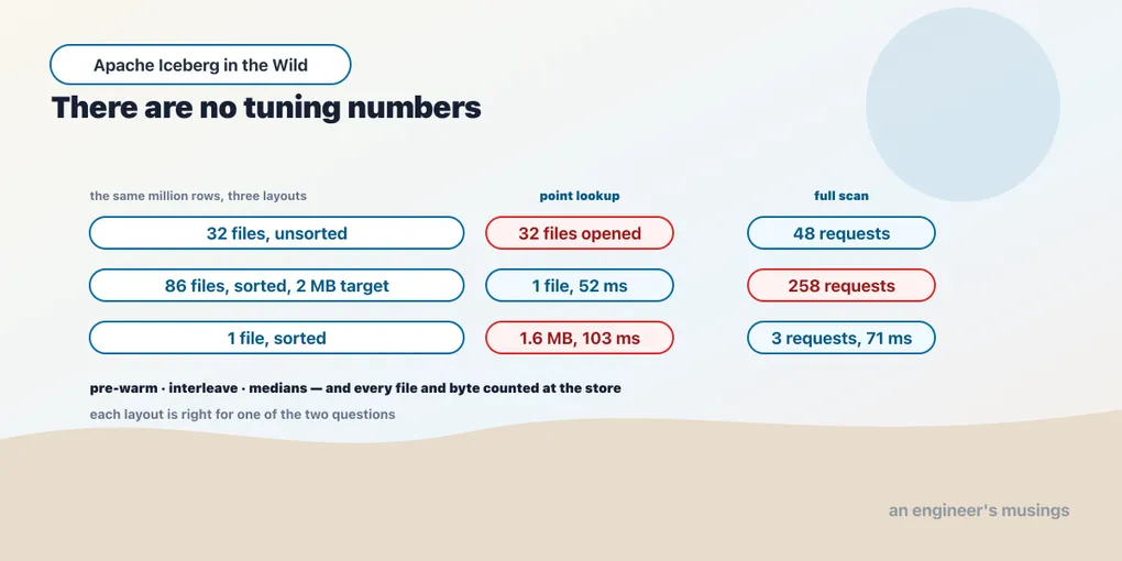
A million-row customer dimension, sixty columns wide, laid out three ways and asked two questions. The first question is a point lookup by customer_id. The second is a filter on two attribute columns over every row.
| Layout | Point lookup: files opened, bytes, median | Two-column filter: files opened, bytes, median |
|---|---|---|
| 32 files, unsorted | 32, 0.4 MB, 82 ms | 48 requests, 1.4 MB, 96 ms |
| 86 files, sorted, 2 MB target | 1, 0.0 MB, 52 ms | 258 requests, 7.1 MB, 230 ms |
| 1 file, sorted | 1, 1.6 MB, 103 ms | 3 requests, 1.8 MB, 71 ms |
The second layout is the one every guide to Iceberg performance would tell you to build for the point lookup, and it does win the point lookup. One file opened instead of thirty-two, nothing fetched but a footer, half the latency. It also makes the full scan two and a half times slower, because a query that touches every file now touches eighty-six of them. The third layout fixes the scan and gives the lookup back its latency, because a single sorted file has to read a whole row group to find one row. None of the three is wrong. Each is right for one of the two questions.
That is the chapter. There are no tuning numbers — only workloads — and a table design is a bet about which questions the table will be asked. The bet can be measured before it is placed, and this chapter is about how to measure it so that the number you write down is the number a reader gets.
The protocol, before the numbers
Book 1 published a copy-on-write versus merge-on-read comparison as “less than half the time” and later retracted it. The first measurement in a JVM session is warm-up, the “before” arm is always measured first, and the 2.3× was the cost of class loading wearing the costume of a write mode. Re-measured properly it was 1.15×. Every timing in this book uses the protocol that retraction produced, and it fits in a dozen lines.
def bench(label, arms, rounds=7, warm=2):
    for name, fn in arms.items():
        for _ in range(warm): fn()                 # pre-warm every arm
    times = {n: [] for n in arms}
    for _ in range(rounds):
        for name, fn in arms.items():             # interleave: A, B, A, B, …
            t = time.perf_counter(); fn()
            times[name].append((time.perf_counter() - t) * 1000)
    # report the median and the spread, never the first run
Three rules, each one earned. Pre-warm every arm, so that class loading and the first metadata fetch are paid before the clock starts. Interleave the arms, so that whatever drifts during the run — a garbage collection, a background compaction, the object store’s own cache — drifts on both equally. Report the median and the spread, so that a reader can see when two arms overlap and the difference is noise.
Latency is the weakest of the four numbers this chapter reports, and it is reported last. The other three come from the counting proxy chapter 2 introduced: how many data files a query opened, how many bytes it fetched, and how many requests that took. Those do not care whether the JVM is warm. They are properties of the layout, and they are the numbers the bill is made of.
The pins: Spark 4.1.3 on the host with local[4], Iceberg 1.11.0, the reference REST catalog on SeaweedFS, every S3 call through the proxy. Rows are the bookshop’s, generated to size.
Workload one: append-only events
Two million events over nine days from five hundred customers, written once. Design A is the table anyone gets by default: no partition, no sort. Design B is partitioned by day and, within each write, sorted by customer_id.
  A unpartitioned/unsorted:           4 files,  9.4 MB, written in 3.0s
  B day-partitioned + sorted:        12 files,  4.8 MB, written in 2.5s
Before either query runs, Design B already has a storage advantage: the sorted table is half the size. Same rows, same Parquet, same compression codec — sorting by customer put similar values next to each other and the encoders did the rest. Design B was also faster to write, because Spark’s sort happens in memory before the files are cut and the smaller files are cheaper to upload. That halving is free and it is the reason to sort even a table nobody ever filters.
Then the two questions the bookshop asks of an events table.
| Query | A: files, bytes, median | B: files, bytes, median |
|---|---|---|
| One day’s revenue | 12 requests, 7.2 MB, 209 ms | 6 requests, 0.2 MB, 110 ms |
| One customer’s events | 16 requests, 7.7 MB, 154 ms | 36 requests, 1.1 MB, 119 ms |
The day query is partition pruning doing exactly what Book 1’s chapter 8 said it would: B opens one partition’s files and fetches a fiftieth of the bytes. The customer query is the interesting row. B makes more requests than A — thirty-six against sixteen — because the customer’s rows are spread across nine day partitions and each one has to be opened. It fetches seven times fewer bytes, because within each day the sort put that customer’s rows in one row group and the statistics let the reader skip the rest. On a store that prices requests and bytes separately, that row is a real trade, and chapter 2’s request table is how you price it. On latency, B wins by a quarter.
Design B is the right answer for this workload, and the rule it illustrates is general. Partition by what you filter on most, sort by what you filter on next, and expect the sort to pay for itself in storage before it pays in queries.
Workload two: upsert-heavy orders
A million orders, and five rounds of MERGE INTO that each update one percent of them — the shape of a nightly reconciliation against an operational system. Design A is copy-on-write, where an update rewrites every file that contains a changed row. Design B is merge-on-read, where an update writes the new rows and a delete file marking the old ones, and readers merge the two. Both tables are bucketed eight ways on order_id so that the merge’s join has somewhere to go.
The merges themselves, one warm-up round and then five interleaved.
MERGE 1% (5 interleaved rounds) cow: median 1014 ms (950–1105) mor: median 762 ms (725–851)Merge-on-read is a third faster to write, and the spreads do not overlap. That is the expected direction; Book 1’s retracted number was the same direction with the wrong magnitude. What the write time does not show is what the two designs did to the table.
  orders_cow: 8 data files, 0 delete files
  orders_mor: 56 data files, 8 delete files holding 60,000 deleted positions
Copy-on-write left the table as it found it: eight files, one per bucket, each rewritten five times. Merge-on-read left fifty-six data files and eight delete files, because each merge added a file of new rows per bucket and marked sixty thousand old positions for deletion. Now read the table.
read after 6 merges cow: 24 requests, 109 ms mor: 192 requests, 239 msEight times the requests and more than twice the latency, for a query that groups a million rows by status. Every reader of the merge-on-read table has to open every data file and apply every delete file that touches it, on every query, until somebody compacts.
  rewrite_position_delete_files   0.1s -> (0, 0)
  rewrite_data_files              0.7s -> (56, 8)
  mor after compaction: 8 data files, 8 delete files still listed, read now 24 requests
  read after compaction   cow: median 112 ms     mor: median 105 ms
One compaction and the merge-on-read table reads like the copy-on-write one. Two details from that run belong in chapter 8 but are worth seeing here. rewrite_position_delete_files did nothing, because there was nothing to merge — eight delete files, one per bucket, is already the minimum. And after compaction the eight delete files are still listed in the metadata, exactly as Book 1’s chapter 12 found. They reference data files that no longer exist in the current snapshot, so readers ignore them, and they stay until snapshot expiry removes them. The read cost is gone; the file count is not.
The design decision is a schedule — not a mode. Merge-on-read when writes are frequent and reads can wait for a compaction, with the compaction scheduled against the write cadence. Copy-on-write when reads dominate and updates are rare or small, so that the table is always in its compacted state and no job has to keep it there. The exception is a table updated by a stream, which cannot be copy-on-write at all; chapter 11 is that table.
Workload three: the wide dimension
A million customers with sixty columns, written in eight batches. Design A is unsorted. Design B declared WRITE ORDERED BY customer_id, which is what the documentation suggests for a table looked up by key. Both came out at thirty-two files and 5.9 MB.
  point lookup by customer_id     dim_a: 32 requests, 0.4 MB, 91 ms    dim_b: 32 requests, 0.4 MB, 92 ms
  3-column projection, all rows   dim_a: 128 requests, 0.4 MB          dim_b: 128 requests, 0.4 MB
  2-column filter, all rows       dim_a: 48 requests, 1.4 MB, 96 ms    dim_b: 48 requests, 1.4 MB, 93 ms
Identical, on every query. The sort order did nothing, and the reason is in how the table was written. WRITE ORDERED BY sorts each write. Each of the eight writes covered the whole range of customer ids, so every one of the thirty-two files has a minimum near zero and a maximum near a million. The statistics that pruning depends on bracket every lookup value in every file. A sort order that holds within a write does not cluster across writes, and clustering across files is what a point lookup needs. This was the first result the harness produced and it was published as written, because it is the mistake a reasonable engineer makes.
Clustering across files means rewriting them, which is a compaction with a sort strategy.
CALL ice.system.rewrite_data_files(table => 'stage9.dim_b',
  strategy => 'sort', sort_order => 'customer_id ASC NULLS LAST')
dim_b after sort compaction: rewrote 32 files into 1 in 6.1s; now 1 file, 5.1 MB
point lookup, B clustered dim_a: 32 requests, 0.4 MB, 82 ms dim_b: 4 requests, 1.6 MB, 103 ms
2-column filter, B clustered dim_a: 48 requests, 1.4 MB, 96 ms dim_b: 3 requests, 1.8 MB, 71 msNow the point lookup opens one file — and is slower. The one file is five megabytes and the row group that holds the customer is 1.6 MB of it, which is more bytes than the thirty-two footers the unsorted table read. The full scan got cheaper in requests and faster in time. And the first attempt at this compaction, with a two-megabyte target file size, produced the middle row of the chapter’s opening table. Eighty-six small sorted files, a point lookup that fetched almost nothing, and a scan that had to open all eighty-six.
The projection is the row that did not move at all: three columns out of sixty, 0.4 MB out of 5.9, in every layout. Column pruning is Parquet’s, not the layout’s, and it is the reason a sixty-column dimension costs a three-column query almost nothing whatever else you do to it.
The declared sort order did not separate customer ranges across batches; the rewrite did. Cluster by rewriting, not by declaring, and choose the target file size for the query you will run more often. Small files for lookups that must fetch little; large files for scans that must open little. Chapter 7 goes further into the layout choices, and chapter 8 into the compaction that makes them hold.
The knobs the worksheet turns
Every design above was made with five table properties, and their defaults were read from the 1.11.0 jar rather than from a page that might describe a different release.
| Property | Default in 1.11.0 | What it decided in this chapter |
|---|---|---|
write.target-file-size-bytes | 536,870,912 (512 MB) | why the sorted dimension became one file, and why the 2 MB override became eighty-six |
write.parquet.row-group-size-bytes | 134,217,728 (128 MB) | why a point lookup in the single sorted file fetched 1.6 MB: the smallest unit a reader can skip is a row group |
read.split.target-size | 134,217,728 | how many tasks a scan of one large file becomes |
write.parquet.compression-codec | zstd since 1.4.0, gzip before | the halving of the events table came from the sort, not the codec; both tables used the same one |
write.delete.mode, write.update.mode, write.merge.mode | copy-on-write | the whole of workload two |
The target file size cannot make a small write larger. It is a ceiling on the file a writer produces, so a small write still makes a small file. Only a rewrite brings files up to the target, which is why chapter 8 is about compaction rather than about this property. And the row-group size is the reason the single-file lookup fetched more bytes than the thirty-two-file one. Parquet statistics let a reader skip a row group, never part of one, so the smallest fetch a lookup can make is one row group. At 128 MB that is most of a small table. The eighty-six-file layout won the lookup by making every file smaller than a row group.
Translating a workload into a design
The three experiments give us four questions to answer before choosing a layout: what readers filter on, how data arrives, how quickly readers need it, and how rows change. The platform keeps those answers in a worksheet for each table. Here it is filled in for events, orders and the customer dimension.
| Question | Decides | Events | Orders | Dimension |
|---|---|---|---|---|
| What does the common query filter on? | partition spec, then sort order | day, then customer | order id (bucket) | customer id |
| How does data arrive? | file size, commit cadence, write mode | one batch a day, append only | nightly merge of one percent | eight batches, then rarely |
| What latency does the reader expect? | copy-on-write or merge-on-read, and the compaction schedule | seconds, from a dashboard | seconds, after the nightly merge | milliseconds, point lookups |
| How do rows change? | delete mode, isolation level (chapter 4) | never | updated in place | replaced in bulk |
| Design | day partition, sorted by customer, single writer | bucket(8, order_id), merge-on-read, compact after each merge | unpartitioned, sort-compacted into one file per few hundred thousand rows |
Two habits make the worksheet more than a form. Fill it in from the query log — not from the schema. The events table’s sort key is customer_id because the second most common filter is a customer, and nothing in the schema says so. And measure the design against the worksheet’s own queries before the table goes live, with the harness. The wide dimension’s declared sort order looked right on the worksheet and did nothing on the table.
What was not run
The numbers are from tables of a few million rows on one machine with a local object store. That is enough to show the shape of every trade-off — and not enough to put a dollar figure on any. Nothing here was priced against a real S3 bill; chapter 18 does that. No table exceeded memory, so the scans are all cached-data scans and a cold read from a remote store will widen every gap. Z-ordering, which chapter 7 covers, was not compared against the plain sort. And every query ran alone; concurrent readers, which change what “fast” means on a shared platform, are chapter 13’s territory.
Exercises
1. Break the sort the other way. Rewrite the events table with WRITE ORDERED BY customer_id but write it in one batch instead of one per day. Then run the customer query and count files opened. Explain the number using the file statistics from the files metadata table.
Show answer
One batch sorted by customer produces files with disjoint customer ranges, so the customer query opens one file per day partition at most and usually fewer. The lower_bounds and upper_bounds columns of files show non-overlapping ranges for customer_id, which is the property the eight-batch dimension lacked.
2. Find the break-even. For the orders table, vary the merge size from one percent to ten percent of rows and re-run the interleaved merge benchmark. At what update fraction does copy-on-write stop being slower to write than merge-on-read, and why does the read cost of merge-on-read not depend on that fraction at all?
Show answer
Copy-on-write cost scales with the number of files touched, and at some fraction every file is touched either way, so the two write costs converge. Merge-on-read’s read cost depends on the number of delete files and data files present, which grows with the number of merges, not with their size. A large merge favours copy-on-write; many small merges favour merge-on-read with a compaction schedule.
Final thoughts
The wide dimension was laid out three times and each layout won one question and lost another. The events table halved in size from a sort nobody asked for. The merge-on-read table was faster to write, slower to read, and equal to copy-on-write after a compaction. Not one of those results is a tuning number that transfers to your table — and every one of them came from the same twelve-line protocol that anyone can run against theirs.
The next chapter takes the layout question deeper, into partition transforms, bucketing, skew and what happens to a good layout when the access pattern under it changes.
Comments