LoRA: Train Less, Learn More

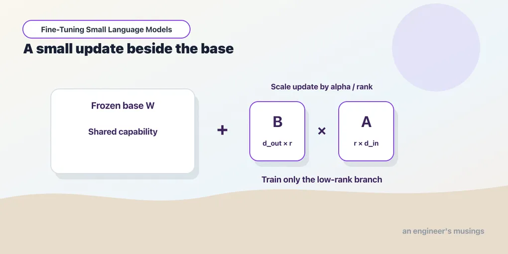
A full checkpoint carries every trained weight, even when the new task is only choosing one of five destinations. That becomes expensive to store and distribute when several teams need different narrow behaviors from the same base model. LoRA is the answer to that cost: it keeps the task-specific change in a separate adapter.

Low-Rank Adaptation keeps the base weights frozen and learns small matrices alongside selected linear layers. The resulting adapter depends on the original base — it is a compact description of a task-specific update, not a standalone language model.

The bookshop comparison uses the same 150 requests and the same fresh evaluation as full fine-tuning. It changes which parameters may learn and uses a larger learning rate for the adapter, so we compare two specified recipes. On the author’s machine, the adapter trained in about forty seconds and matched the full fine-tune on every test request. Its saved directory occupied 19.54 MiB instead of about 2.2 GiB. Those are the recorded results to inspect; your own run needs its own timing and predictions.

Run against: PEFT 0.17.1, PyTorch 2.8.0, Transformers 4.56.2, pinned Qwen3-0.6B on Apple M1 Ultra/MPS; rank 8, alpha 16, query/value projections, float32, dataset router-v2, plan training-v2. The printed progress lines and result fields are from the recorded LoRA run’s log and results.json.

Not run. Alternative ranks and target-module sweeps, adapter composition, concurrent adapter serving, and cross-device merge equivalence are outside this experiment.

Replace a large update with two smaller factors

A linear layer multiplies its input values by a matrix of weights. A matrix arranges numbers in rows and columns, and its shape gives the count of each. Call this weight matrix W. Full fine-tuning can change every entry in it. LoRA keeps it frozen and learns an addition made from two smaller matrices, called factors. The equation below adds that learned contribution to the base. Alpha controls its scale, while the rank sets the size of the intermediate representation inside the adapter:

W_effective = W + (alpha / r) × B × A

If W has shape d_out × d_in, its row count is the number of output values and its column count is the number of input values. Then A has shape r × d_in: it takes the input into a smaller intermediate representation. Next, B has shape d_out × r and brings that representation to the required output size. Their product has the same shape as W, so it can contribute to the same output, and the rank r sets the intermediate width.

Full training exposes d_out × d_in parameters for the layer; LoRA exposes r × (d_in + d_out), the entries in the two factors. We never form a dense update and compress it afterwards.

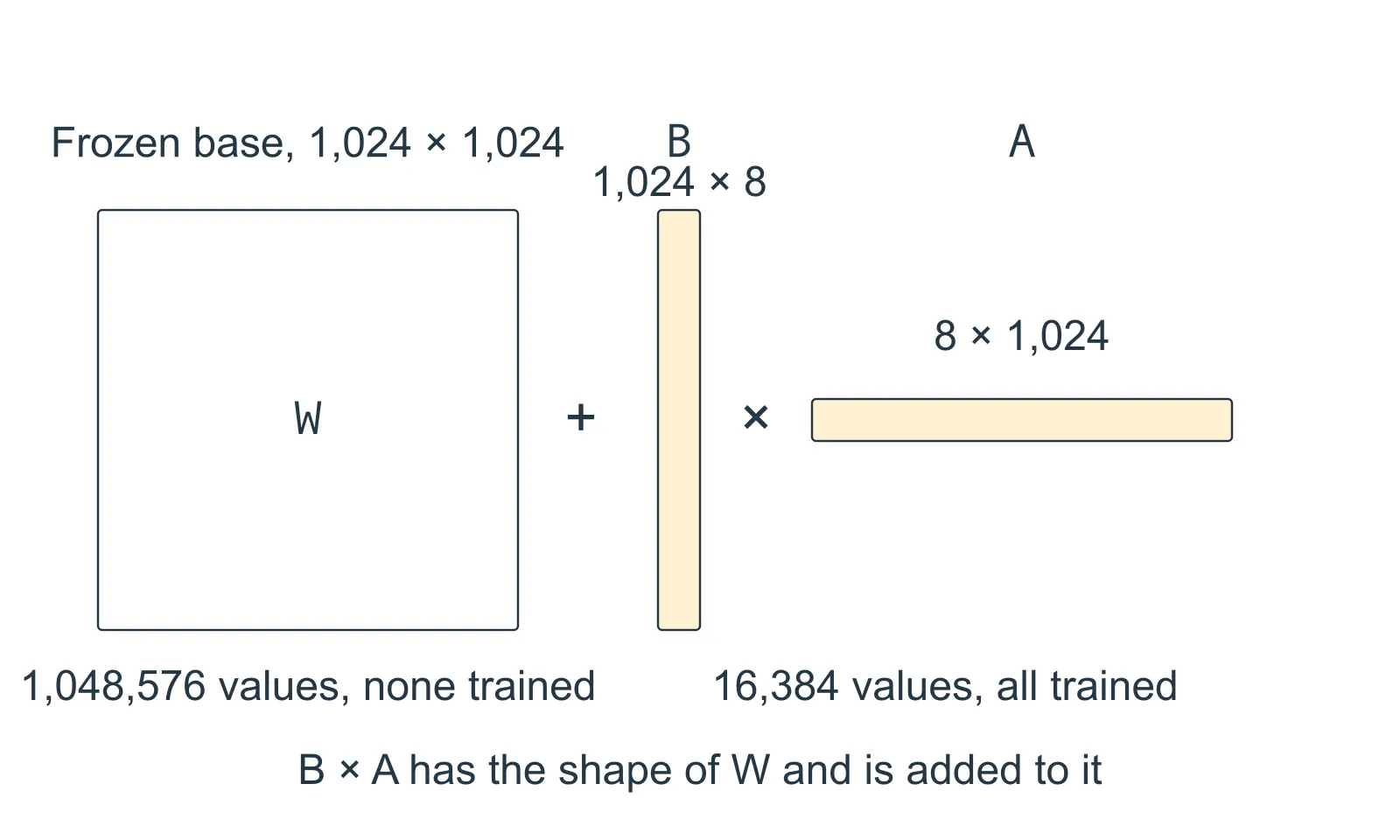
Figure 08.1. The boxes are drawn to their shapes: the thin factors share the long dimension of W and have a width of eight, the rank. Every entry of the product can differ from zero, but the product is built from 16,384 learned values rather than a million. Amber marks the trainable factors.

Rank limits the space of possible updates without saying that only eight original weights may change. For the square 1,024-by-1,024 projection in Figure 08.1 with rank eight, the factors together contain 16,384 trainable values, while their product B × A has 1,048,576 entries. Those entries are determined by the factors rather than learned independently. The product can therefore touch every output-input pair while staying confined to a low-rank structure. That is how a small adapter can alter behavior broadly without learning a separate value for every pair.

The scaling factor controls the contribution of the learned branch. In this recipe alpha is sixteen and rank is eight, giving a factor of two. Changing the rank while leaving alpha fixed also changes that scale under the standard formula — so a rank comparison needs an explicit scaling policy if it is meant to isolate capacity. The original LoRA paper motivates low-rank updates as an efficient way to adapt large models. Our experiment tests one configuration on one task.

Work through one low-rank branch

A small numerical example makes those dimensions concrete. Let a frozen two-by-two base weight be the identity matrix, which returns its input unchanged. Let the rank-one factors be A = [1, 2] and B = [0.1, -0.2] as a column, with scaling one. The first factor is a row; the second stacks its values vertically. Multiplying each value in the column by the row gives this two-by-two update:

B × A = [[ 0.1,  0.2],
         [-0.2, -0.4]]

For input [3, 4], the base returns [3, 4]. The adapter first computes A × input = 11 by multiplying corresponding entries and adding the products. It then multiplies that single value by each entry of B, yielding [1.1, -2.2]. Adding these adjustments to the corresponding base outputs gives [4.1, 1.8]. The merged effective matrix is the base matrix with the update added to it. Multiplying the input by that combined matrix gives the same result.

Notice that the update changed both output coordinates even though its internal representation has only one dimension. That is what rank one constrains — the update travels through a single intermediate direction — and it does not restrict the model to changing one output element. Increasing the rank gives the update more independent directions and more parameters to fit from the same examples; whether that helps depends on the task.

The branch also explains switching. Keeping the base fixed and selecting another pair of factors changes the task-specific contribution, which is why one cached base can serve several specialists. The application still has to select the right policy and tokenizer behavior with each adapter. A server that attaches the wrong adapter returns valid labels under the wrong business boundary — an error harder to notice than a crash.

Freeze weights without severing the computation

A frozen base parameter has no gradient buffer and its value never changes. The forward pass still uses it, though, and backward still needs enough of the computation to find gradients for the adapter parameters. Freezing most weights therefore removes their optimizer state and parameter-gradient storage. It does not remove the activations, and it does not shrink the architecture to a tiny independent network.

PEFT’s standard initialization makes the initial adapter contribution zero by initializing one factor to zeros, so the adapted model begins with exactly the base transformation at the targeted layers. That is not the same as two zero factors. If both were zero, each factor’s gradient through the product would depend on the other zero factor, and nothing could start learning. Keeping one factor nonzero preserves a gradient path while starting from the base behavior. The printed losses below show this initialization at work.

The companion watches the first query projection and its two adapter factors. An unchanged base tensor says the frozen weight stayed frozen; changed factors say learning reached the adapter. Neither check replaces held-out predictions, but together they catch a job that trained the wrong parameter set.

Choose the layers that can express the task

A language model like Qwen is a stack of repeated layers, and every token position passes through all of them in turn. Each layer has two parts. An attention block lets a position gather information from the positions before it — this is how the label position can use the policy and the request — and a feed-forward block then transforms what was gathered. The attention block does its work through linear projections, and three of them matter here: the query projection, q_proj, decides what a position looks for; the key projection decides what each earlier position offers; the value projection, v_proj, carries the information that is combined. The recipe attaches adapters to q_proj and v_proj in every layer, which gives the router a small starting configuration. Keys, attention output projections and feed-forward projections can also be adapted, at a larger parameter and optimizer cost, and a result from query/value adaptation describes that configuration rather than LoRA in general.

The configuration collects the rank, scaling and layer choices just described. Dropout is an additional training control that randomly leaves out some values; this recipe turns it off. The task type keeps the next-token prediction objective used for the router:

config = LoraConfig(
    r=8,
    lora_alpha=16,
    lora_dropout=0,
    target_modules=['q_proj', 'v_proj'],
    task_type='CAUSAL_LM',
)
model = get_peft_model(model, config)

Qwen’s projection dimensions are not all the same: its key and value projections are narrower than its query projection. Counting a fictional square matrix for every target therefore gives the wrong total. The actual PEFT model reports 1,146,880 trainable parameters for this rank-eight query/value configuration — the number Chapter 4’s smoke test printed.

Zero dropout removes a source of randomness from this small comparison; it is not a general recommendation against it. And before reusing a familiar configuration on another model, inspect which modules it matched and the trainable count it produced. Module names belong to an architecture: the same configuration string on another family may match nothing, select different layers, or need extra saved modules.

Train the adapter

The command differs from Chapter 7’s by one word: the mode selects adapter training. It uses the same prepared environment, and the directory must again be new. The recorded output below also lets you follow the comparison without running another training job:

.venv/bin/python train_router.py \
  --mode lora --size 150 --epochs 2 \
  --output runs/local-lora \
  --evaluate test --reload

The run prints the same progress lines as the full fine-tune. These are the recorded run’s:

lora 150 {'step': 1, 'epoch': 0, 'loss': 0.7232056856155396} elapsed 0.99
lora 150 {'step': 10, 'epoch': 0, 'loss': 0.16325759887695312} elapsed 5.71
lora 150 {'step': 20, 'epoch': 0, 'loss': 0.0038976820651441813} elapsed 10.96
lora 150 {'step': 30, 'epoch': 0, 'loss': 0.11883704364299774} elapsed 16.21
lora 150 {'step': 40, 'epoch': 1, 'loss': 0.1318548619747162} elapsed 21.61
lora 150 {'step': 50, 'epoch': 1, 'loss': 0.020028429105877876} elapsed 26.86
lora 150 {'step': 60, 'epoch': 1, 'loss': 0.0012665684334933758} elapsed 32.11
lora 150 {'step': 70, 'epoch': 1, 'loss': 0.0012490653898566961} elapsed 37.36

Put Chapter 7’s first line beside this one. The full fine-tune’s first batch scored 0.7232056856155396, and so does the adapter’s — the same twelve digits. That is the zero initialization made visible. Before the first update the adapter contributes nothing, so the model is numerically the base model, and the same seed gives it the same first batch. From the second step on, the two runs part company. By step 10 the adapter is at 0.16 where the full run was at 1.31, and its last recorded value in loss.jsonl is 0.00054. The noise is still there — step 40 is higher than step 20 — but the trend is cleaner than the full run’s. Each step takes about half a second against the full run’s three quarters.

The run then evaluates the candidate and reloads the saved adapter onto a freshly loaded base. It also merges the adapter contribution into the base weights, as in the numerical example, and prints its results.json. The equality fields below report whether those reconstructed candidates preserve the predicted labels:

"optimizer_steps": 76
"training_seconds": 40.28093908401206
"accuracy": 1.0
"macro_f1": 1.0
"reload_predictions_equal": true
"merged_predictions_equal": true

Compare it with full fine-tuning

Both arms see two passes over the same 150-row core, with batch size four and seed 42, AdamW, weight decay 0.01 and clipping at norm 1.0. Both fix their final checkpoint in advance rather than selecting it by the test. The learning rates differ — 2e-5 for full training and 2e-4 for LoRA — because adapter training optimizes a different structure. Those values are declared choices rather than the winners of a search, so the comparison is between complete recipes, and it does not pretend that every numerical condition is identical.

The test is the same fresh fifty-row fixture, with no demonstrations in the prompt for either candidate. Combining a trained adapter with twenty-shot prompting could be useful, but it would need its own measured arm.

Method	Accuracy	Macro-F1	Trainable parameters	Training seconds	Saved directory MiB
full	100%	1.000	596,049,920	59.51	2288.93
lora	100%	1.000	1,146,880	40.28	19.54

Both candidates get all fifty test requests right with no invalid outputs. That is an observed tie at the fixture’s ceiling, not proof of equivalent generalization. The saved confusion matrices and raw predictions are what to read when two candidates tie, because aggregate accuracy can match while the models fail on different requests. LoRA completes its 76 updates in 40.28 seconds against 59.51 for full training, in single local runs.

The adapter exposes about 0.192% as many trainable parameters as the full model. Its saved directory is 19.54 MiB because tokenizer files travel with the adapter weights and configuration; the adapter tensors themselves are about 4.38 MiB at float32. The watched base query projection is unchanged, both watched adapter factors changed, and the reloaded and merged candidates both reproduce all fifty labels.

The memory counters need their scopes stated. After training, the MPS allocation snapshot is about 2,284.82 MiB for LoRA against 4,893.32 MiB for full training. The runner takes this snapshot after deleting the optimizer and saving the candidate, so it measures tensors retained at that point. It does not measure the optimizer state held during training; that theoretical saving is discussed below. Process peak RSS moves the other way, about 5,212.05 MiB for LoRA against 4,837.77 MiB for full. The LoRA process did more after training — it reloaded and merged the adapter and evaluated both — which is a plausible contributor, but the record does not isolate it. The RSS values cover a different scope and cannot be relabeled as peak accelerator memory or used to contradict the allocation snapshot.

Three conclusions come out of the table, and they have different strengths. A smaller artifact is a direct consequence of saving adapter tensors rather than the base. A quality tie is an empirical result on these fifty cases. A timing difference is local to this implementation, hardware and short-sequence workload. They should not be bundled into one claim that LoRA is simply “better.”

Read memory savings without expecting miracles

Full AdamW training needs optimizer state for nearly six hundred million parameters; the adapter optimizer needs it for roughly 1.15 million. That is the saving, and it is large. What it does not touch is the frozen float32 base, which still occupies about 2.22 GiB in parameter tensors — the base does not vanish because its optimizer state did. Nor does it touch the activations that backward needs, which grow with batch size and input length rather than with trainable parameters.

That is why the trainable-parameter ratio predicts the parameter-gradient and optimizer-state reduction and nothing else. Training speed has the same shape. LoRA avoids computing and storing gradients for the frozen base, but it still runs the base forward path and backpropagates through the relevant operations. On short sequences, small matrix multiplications and framework overhead can limit the benefit. The measured forty seconds is more useful than a prediction from parameter counts.

Save the dependency, not just the small file

An adapter save contains adapter weights and configuration, and nothing else. A reproducible deployment therefore needs the exact base model revision, the tokenizer configuration, the adapter, the routing policy and the decoder settings together. Loading an adapter onto a different base revision can succeed mechanically — the tensor shapes match — while changing behavior, because the learned update no longer means the same thing against different base weights. The checkpoint identifier and revision hash are part of the artifact contract, not annotations for a README. The runner pins the base revision explicitly when it rebuilds the model for the reload check.

The saved adapter also contains no training state. AdamW’s running estimates belong to the training job, so exact resumption needs more than the inference adapter, as with the full checkpoint. And a small file invites casual copying between experiments, where naming alone is weak protection. The run manifest should identify the base revision, data hashes, target modules, rank, scaling and seed — that is what distinguishes two artifacts that share a filename.

Storage accounting should also distinguish incremental bytes from the complete runnable package. If ten specialists share one cached base, their incremental storage is small; if every deployment copies the base into an isolated environment, the saving is different. The companion’s artifact_bytes counts everything written to the directory, tokenizer files included, which is why it is larger than the 4.38 MiB tensor estimate. Reporting both keeps a reader from treating a four-megabyte matrix as the size of the saved directory.

Merge when the deployment actually benefits

For an ordinary floating-point base, the adapter update can be added into the base weight. PEFT’s merge_and_unload() produces a model without separate adapter branches by applying the effective-weight equation directly. That can simplify serving a fixed specialist. It also turns a small dependent artifact into a full model artifact if the merged weights are saved, so switching to another specialist then means another merged model or a reconstruction of base plus adapter.

The companion reloads the adapter, evaluates it, merges it, and evaluates again, and the assertion compares destination labels on the same fifty requests. Matching labels verify the routing behavior of this merge in this environment; floating-point operation order can still move the token scores slightly, so label equality should not be promoted to bitwise equivalence.

A merge is not adapter composition. Adding two independently trained updates assumes their combined behavior stays useful, and they can conflict, especially where both touch the same routing boundaries. Keeping the unmerged adapter preserves the original combination, keeps the merged checkpoint from becoming the only surviving representation, and keeps the experiment that justified a deployment traceable.

Distinguish capacity problems from data problems

When an adapter underperforms, rank is a tempting knob. Ask first whether the training examples teach the decision it missed: a mislabeled example stays mislabeled at every rank, and a larger update matrix cannot supply a missing boundary. Once the supervision is checked, rank and target modules become useful experiments. Adapting all linear layers is one of them — more freedom at a larger parameter and optimizer cost — and the comparison should hold data and evaluation fixed and record any learning-rate change.

Training loss and held-out errors help separate the possibilities. High training loss suggests inadequate optimization, insufficient capacity or an interface defect; low training loss with poor held-out behavior points at generalization or coverage. Neither pattern is a complete diagnosis, but both say which controlled experiment comes next.

There is also a task-design limit no rank can lift. If the label depends on current inventory, the router should learn to identify the need for a database, not memorize today’s count. An adapter that learns a few inventory facts can look helpful in a demonstration and be stale the next morning. The source boundary stays part of the application design, however efficiently the model adapts.

Exercises

1. Count a low-rank update

A weight has shape 2,048 by 1,024. With rank eight, how many trainable values does its LoRA update contain, excluding bias?

Answer

8 × (2,048 + 1,024) = 24,576. Full training of that matrix exposes 2,048 × 1,024 = 2,097,152 values. The low-rank product can affect every effective matrix entry despite using far fewer independent values.

2. Diagnose two zero factors

Why would initializing both A and B to zero prevent the adapter from learning through their product?

Answer

The gradient for each factor depends on the other factor. With both zero, the product’s gradients for both factors are zero. Standard initialization keeps one factor nonzero while making the initial product zero, preserving an initial gradient path.

3. Explain a memory surprise

The adapter has hundreds of times fewer trainable parameters, but process peak memory falls by much less. What still occupies memory?

Answer

The frozen base weights, activations needed for backward, temporary buffers, framework state, and loading/evaluation allocations remain. Trainable-parameter count mainly predicts the parameter-gradient and optimizer-state reduction, not every component of process memory.

4. Define a deployable adapter

A colleague sends only adapter_model.safetensors. What else must be identified before treating it as a reproducible router?

Answer

The adapter configuration, exact base model and revision, tokenizer and chat-template settings, policy, label parser, generation configuration, and compatible runtime are required. The small tensor file alone does not define the complete behavior.

Final thoughts

If your environments already share a base model, LoRA makes the specialist cheap to store and easy to move between them. That separation of common capability from task-specific change is its strongest practical benefit. We still have to earn the quality on the task, and the frozen base still takes memory — which is the constraint four-bit storage addresses next.

Next: QLoRA: Fine-Tuning Under Memory Constraints