Your First Full Fine-Tune

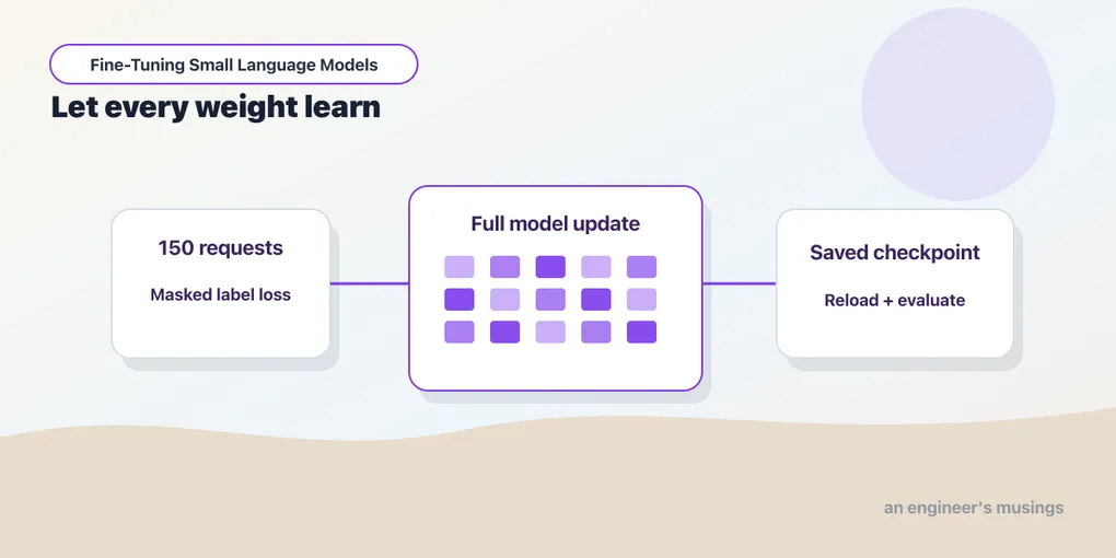
A falling training loss is encouraging, but we still need to see where the router sends unfamiliar orders. It may be learning to complete the training requests without becoming useful beyond them. That is why our first fine-tune has to leave us with three things: a saved checkpoint, a fresh evaluation, and an explanation of what changed.

Full fine-tuning makes every original model parameter eligible for an update. Chapter 3 changed one weight; here the same prediction, loss, and update process involves the model’s many weights. Giving the optimizer that freedom also means keeping gradients and optimizer state for far more values than an adapter method needs.

The bookshop experiment starts with Qwen3-0.6B and the 150-request core from Chapter 6, and it keeps the routing policy, the exact-label parser, non-thinking generation and the twelve-token output budget. The inference prompt contains the policy and the request with no demonstrations, so training has to earn any improvement under that interface.

Run against: Qwen/Qwen3-0.6B revision c1899de289a04d12100db370d81485cdf75e47ca; Python 3.13.3, PyTorch 2.8.0, Transformers 4.56.2, Apple M1 Ultra/MPS, float32 and eager attention; companion train_router.py, dataset router-v2, plan training-v2. The printed progress lines and result fields are from the recorded full run’s log and results.json. The standard-library loss and saved-result activities were checked with Python 3.13.5.

Not run. CUDA training, distributed training, mixed-precision training, multiple random seeds, and production-quality evaluation are outside this experiment.

Understand the prediction before the update

The model reads a system policy and a user request through its chat template, and at the assistant boundary it predicts destination tokens. The supervised target is the correct label followed by the end token, so a wrong label means the model assigned too little probability to the desired completion under that context.

For one desired token, cross-entropy loss is the negative natural logarithm of the probability assigned to that token. Python’s math.log calculates the natural logarithm. Try these supplied probabilities with your existing Python installation; no model is involved:

import math

for probability in (0.1, 0.5, 0.9):
    loss = -math.log(probability)
    print(f"Target probability {probability:.1f}: loss {loss:.3f}")

Target probability 0.1: loss 2.303
Target probability 0.5: loss 0.693
Target probability 0.9: loss 0.105

Giving the desired token more probability reduces its loss. The training code averages these contributions over the scored positions from Chapter 6. A loss of 0.693 is not 69.3 percent wrong answers: loss measures token probabilities, while routing accuracy counts complete labels that match the expected destination.

That distinction matters for a multi-token label. A model can become more confident about the shared prefix of a destination while still getting the decisive token wrong. It can also lower the loss on examples it already answers correctly without fixing a single wrong route. Exact-label predictions remain the task metric; loss is a diagnostic of the training process.

The model performs the next-token shift internally, as Chapter 6 described. Input tokens occupy their normal sequence positions, and the label sequence carries the same target token IDs at the supervised positions. Shifting the labels by hand before passing them in would shift them twice and teach the wrong next-token relationship.

The -100 mask excludes the supplied policy and request from the loss. Their tokens still take part in the forward computation and shape the internal state from which the label is predicted. Ignoring their loss does not make them invisible to attention, the mechanism by which each position draws on the tokens before it — which is exactly why completion-only training can learn to use the request without spending its objective on reproducing it.

Put two different lengths in one batch

Chapter 6 built two lists for one row, input_ids and labels, and stopped there. Training processes examples in groups called batches, and to arrange several rows’ token lists into one rectangular array, called a tensor, every row has to be the same length. Padding fills the unused positions at the right of a shorter row, and that is where a second mask enters.

Take Chapter 6’s toy row, with the prefix [11, 12, 13], the destination [41, 42] and the end token 99. Now suppose a second request has the shorter prefix [11, 14] with the same completion. The first sequence has six tokens and the second has five, so for this illustration the second is padded to six:

Second row’s position	1	2	3	4	5	6
Token’s role	Prefix	Prefix	Label part 1	Label part 2	End	Padding
input_ids	11	14	41	42	99	99
labels	-100	-100	41	42	99	-100
attention_mask	1	1	1	1	1	0

The attention mask marks real sequence positions with 1 and padding with 0, so padding is excluded as context. The first row needs no padding here, so its attention mask is six ones. The loss mask does a different job: it selects which target positions are scored. A prefix position has attention value 1 but target value -100, which reads as “use this as context, but do not score its reproduction.”

Notice the two 99 values at the end of the second input. The first is the real ending and the second fills empty space, because the companion reuses the end-token ID as its padding token. Their positions and masks tell them apart — and that is the trap: replacing every 99 in labels with -100 would erase the real stopping target along with the padding. Count the scored positions in each row before moving on. Both have three, two destination tokens and one real end token, and the padding contributes none.

The actual runner pads every batch to a fixed width of 256 tokens rather than the six used here. It rejects any encoded prefix plus completion longer than that instead of silently cutting text off. Every request in this fixture fits. The section on inspecting an update, below, explains why the recorded run uses a fixed width rather than padding each batch to its longest row. Longer real requests would need a deliberate choice between shortening inputs and raising the budget, because losing the decisive phrase or the desired answer changes what an example teaches.

Make the first experiment deliberately ordinary

An epoch is one pass through the training dataset, and an optimizer step applies one update to the trainable parameters. We group four examples into a batch, update once from that batch, then move to the next. After one pass, we shuffle the examples and make a second pass.

Keep the supplied settings for this first experiment. Each controls a different part of that process:

Setting	What it controls	Our choice
Batch size	How many requests contribute to one update	4, with the last smaller batch retained
Epochs	How many passes we make through the training rows	2
Optimizer	How gradients are used to adjust weights	AdamW, which keeps running estimates from earlier gradients
Learning rate	The scale of the optimizer’s update	2e-5, or 0.00002
Weight decay	A separate adjustment pulling weights toward zero	0.01
Gradient clipping	A limit on the combined gradient magnitude	Norm 1.0; larger gradient vectors are scaled down

Chapter 3 used the current gradient directly. AdamW also uses estimates from previous steps to scale its adjustments. Weight decay and clipping are additional controls; neither replaces correct examples or a useful loss. We keep these settings fixed so we can first learn how to run and read one experiment. The final checkpoint after two epochs is the candidate, chosen before test evaluation.

With 150 examples, an epoch has 38 batches — 37 full ones and one batch of two — so two epochs produce 76 optimizer steps. That last partial batch still receives a step of its own. The default token-averaged loss weights each step by its supervised token content, rather than making the whole epoch one exact per-example average.

These choices are a baseline recipe, not a claim of optimal hyperparameters. A small learning rate keeps each full-model update modest, and two passes keep the experiment short; a larger task could need a different schedule or many more examples. What matters is that the settings were fixed before anyone looked at test errors. Changing several of them afterwards would open a new development cycle and need another final reserve.

The seed fixes the initialization of the relevant random state and the order of examples — each epoch uses its own deterministic shuffle. That makes the recipe repeatable enough to investigate without guaranteeing bitwise identity on every accelerator or software version — deterministic intent and cross-platform numerical identity are different claims.

The recorded plan also fixes the LoRA and QLoRA settings for the later comparisons. Their learning rate is larger because they optimize a much smaller parameter subset, so the experiment compares specified training recipes rather than isolating the effect of the method name alone.

Read the saved run first

You can inspect the completed experiment before installing training packages or loading Qwen. From the companion directory prepared in Chapter 4, save this as read_training_result.py and run python3 read_training_result.py:

import json
from pathlib import Path

run = Path("runs/training-v2-full")
result = json.loads((run / "results.json").read_text())
losses = [json.loads(line) for line in (run / "loss.jsonl").read_text().splitlines()]
print("Updates:", result["optimizer_steps"])
print("Recorded losses:", len(losses))
print(f"Test accuracy: {result['metrics']['accuracy']:.0%}")
print("Reloaded labels match:", result["reload_predictions_equal"])

Updates: 76
Recorded losses: 76
Test accuracy: 100%
Reloaded labels match: True

The two counts let us connect the update schedule to its loss record. Accuracy describes the fifty test requests, and the last field checks that saving and reloading preserved their predicted labels. This script only reads files; it does not train or evaluate a model. You can continue with the recorded progress below using those files throughout.

Before a local training run

The supplied train_router.py uses Apple’s MPS device explicitly. Its recorded path needs an Apple Silicon Mac and the frozen training environment; Chapter 4’s CUDA or CPU inference options do not make this training command portable to those devices.

The experiment ran on a machine with 64 GiB of unified memory, which is the tested configuration rather than a minimum; the memory section below works out what the run needs and what it measured. The saved model directory takes about 2,289 MiB of disk space, in addition to the cached base and environment. Readers without a suitable setup can use the saved run.

Run the first fine-tune

Training needs the packages the baseline did not, so install the frozen training requirements into the same environment, then run the recipe. The companion writes to a new output directory and refuses to reuse an existing one. That protects an earlier run’s predictions and configuration from being overwritten — a new candidate needs a new directory even when only one setting changes:

uv pip install --python .venv/bin/python -r requirements-training-frozen.txt
.venv/bin/python train_router.py \
  --mode full --size 150 --epochs 2 \
  --output runs/local-full \
  --evaluate test --reload

The runner prints one line at the first step and one every tenth step after that, with the batch loss and the elapsed time. This is what the recorded run printed:

full 150 {'step': 1, 'epoch': 0, 'loss': 0.7232056856155396} elapsed 1.33
full 150 {'step': 10, 'epoch': 0, 'loss': 1.3072036504745483} elapsed 8.32
full 150 {'step': 20, 'epoch': 0, 'loss': 0.06570335477590561} elapsed 16.09
full 150 {'step': 30, 'epoch': 0, 'loss': 1.0129938125610352} elapsed 23.89
full 150 {'step': 40, 'epoch': 1, 'loss': 0.07502119988203049} elapsed 31.77
full 150 {'step': 50, 'epoch': 1, 'loss': 5.430687451735139e-05} elapsed 39.56
full 150 {'step': 60, 'epoch': 1, 'loss': 0.8278700709342957} elapsed 47.34
full 150 {'step': 70, 'epoch': 1, 'loss': 9.267568384530023e-05} elapsed 55.12

Read the loss column before the time column. It does not fall smoothly: the tenth batch scores worse than the first, the thirtieth sits near 1.0 after the twentieth was near zero. The sixtieth jumps back to 0.83 in the second epoch. And the printed lines miss the largest value of all: step 2, which the runner never prints, scored 7.32 — ten times the first batch — and steps 4 and 5 were still at 2.75 and 3.27 before the run settled. Each printed value is one batch of four requests, and batches differ in difficulty, so the single numbers are noisy by nature. The readable signal is the trend across the two epochs — the near-zero values become the rule rather than the exception. The per-step file the run writes, loss.jsonl, holds all 76 values, and the last five are 0.0051, 1.3439, 0.0000, 0.0001 and 0.0000. That spike at step 73, like the one at step 2, is a real batch the model finds hard, not a sign the run diverged.

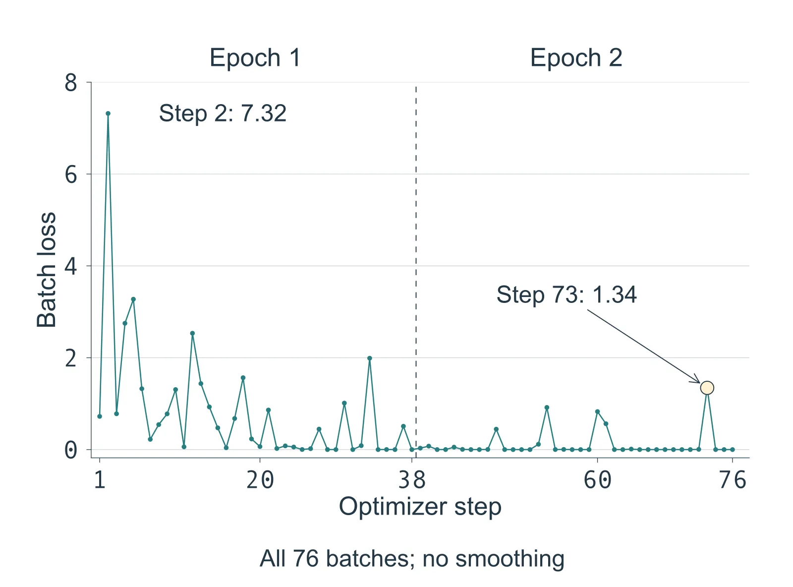
Figure 07.1. Every point is a saved batch loss; the line joins successive observations without smoothing. The dashed line separates two passes of 38 batches. The later losses are usually lower but still spike. This is training loss, not held-out routing accuracy; values close to zero are plotted at their saved precision.

The run finishes by evaluating the candidate, reloading the saved checkpoint, and printing its results.json — these are the fields to look at first:

"optimizer_steps": 76
"training_seconds": 59.50691320816986
"accuracy": 1.0
"macro_f1": 1.0
"reload_predictions_equal": true

Seventy-six steps in just under a minute, every test request routed correctly, and a reloaded checkpoint that reproduces the in-memory predictions. The directory beside it holds the configuration, the per-step loss log, the raw test predictions, that summary, and the model artifact. The summary also records data and runner hashes, parameter counts, timing scopes, memory counters, and the reload agreement. Model weights stay outside the manuscript repository.

Two notes on reproducing it. The recorded environment includes bitsandbytes for the later quantized experiment, which full training does not use. The runner disables optional torch.compile globally so that every method follows the same eager execution plan. Changing the hardware changes both feasibility and speed. The recipe stays inspectable, but a different GPU or service should keep its own metadata and report differences rather than replace the original evidence.

Follow one batch through the loop

Return to Chapter 3’s small update: calculate a prediction, compare it with the target, calculate a gradient, then change the weight. In PyTorch, model(**batch).loss combines prediction and loss calculation, loss.backward() calculates gradients, and opt.step() updates the weights. Before those operations, opt.zero_grad() clears gradients left by the previous batch. A batch replaces the single example, and many weights replace the one number.

The batch supplies both context tokens and desired target tokens. The forward calculation uses the context to predict, and the loss checks those predictions against the unmasked targets. Backward follows that calculation to find how each trainable weight affected the loss. The optimizer then changes the weights, so the next batch starts from the updated model.

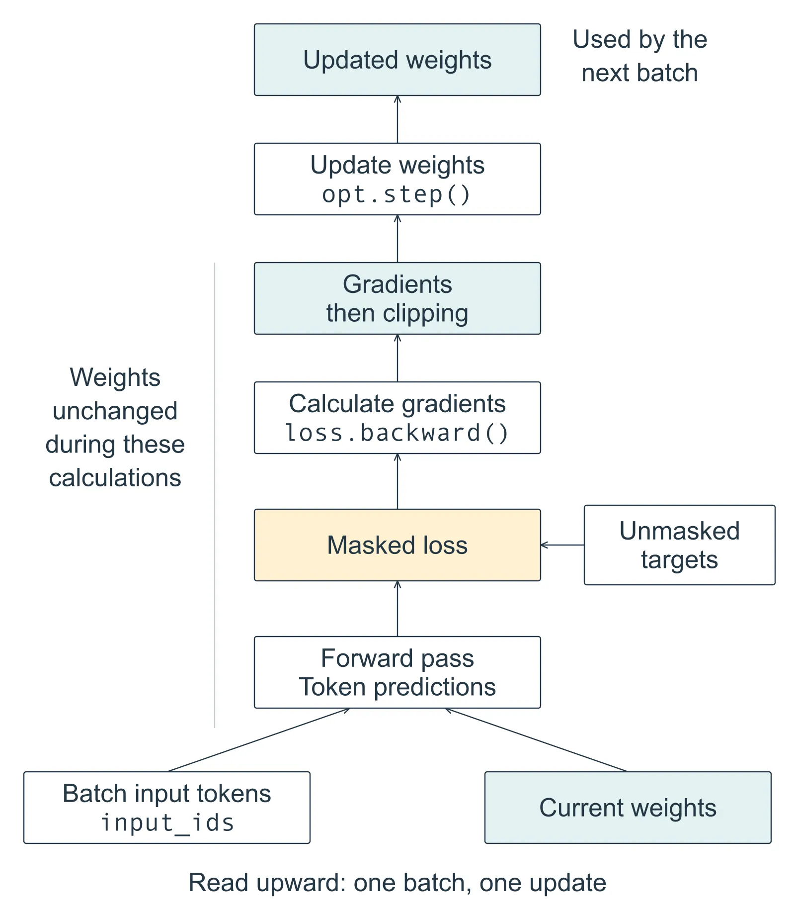
Figure 07.2. Read upward. The batch contributes input tokens and targets with different jobs. Backward calculates gradients through the forward computation; opt.step() is the operation that changes weights. Clear old gradients before starting each batch, as in the loop. The next batch repeats this process using the updated model.

The full loop below surrounds those four jobs with practical work: shuffling the rows, building batches, rejecting a nonfinite loss, clipping gradients, and recording progress. Read the four central operations first, then find where the surrounding work fits. This is the companion loop reformatted for the page, with only the progress print and two bookkeeping lines left out:

model.train(); model.config.use_cache = False
opt = torch.optim.AdamW(
    (p for p in model.parameters() if p.requires_grad),
    lr=meta['learning_rate'], weight_decay=0.01,
)
with (out / 'loss.jsonl').open('w') as log:
    for epoch in range(a.epochs):
        order = list(range(len(data)))
        random.Random(42 + epoch).shuffle(order)
        for i in range(0, len(order), 4):
            batch = collate([encoded[j] for j in order[i:i+4]], tok.pad_token_id)
            opt.zero_grad(set_to_none=True)
            loss = model(**batch).loss
            if not torch.isfinite(loss):
                raise RuntimeError('nonfinite loss')
            loss.backward()
            torch.nn.utils.clip_grad_norm_(model.parameters(), 1.0)
            opt.step()
            sync()
            step += 1
            entry = dict(step=step, epoch=epoch, loss=loss.item())
            log.write(json.dumps(entry) + '\n')

The shuffle is seeded with 42 + epoch, which is how each epoch gets its own deterministic order, and the slice order[i:i+4] is the batch. collate pads the four encoded rows to the fixed width with the end-token ID, as the earlier section described. Everything the progress lines showed comes from entry.

Clearing gradients comes first because PyTorch normally accumulates them; without it, later batches would silently include earlier gradients. set_to_none=True lets the optimizer and autograd tell an absent gradient from an allocated tensor full of zeros.

The forward pass computes the loss. Backpropagation, requested by loss.backward(), works backward through that calculation to find the gradients for the trainable weights — it calculates them, and opt.step() applies the update. Between the two, clipping limits the norm of the gradient vector before the optimizer sees it. AdamW then updates the parameters, scaling each change by its running estimates of recent gradients and their squares, and applies the weight decay from the recipe table as a separate pull toward zero.

Clipping limits the gradient supplied to the optimizer; it does not directly bound the final AdamW weight change. It also cannot fix corrupted labels, a wrong loss mask, or a harmful learning rate. The finite-value check and the loss log give an early signal; the final predictions say whether the task improved.

During training, model.train() enables training behavior and use_cache=False stops the model from keeping the per-token cache that speeds up generation, where each new token is produced from the tokens before it. Backward still needs activations, the intermediate values the forward pass produced. Disabling the cache therefore does not remove training’s activation memory — it removes a separate mechanism meant for generation.

Each step synchronizes MPS before the elapsed time is recorded, because accelerator work is asynchronous and a host timer around a queued operation would understate it. The training timer covers the update loop and its logging; checkpoint saving has a timer of its own, so a slow file write can be told apart from slow optimization.

Read the experiment as a comparison

The unchanged base and the trained candidate receive the same fresh fifty-row test, and they share the policy, the zero-demonstration prompt, the parser, the tokenizer revision and the greedy decoder. The training run uses only the 150-example core for gradients; validation supplies a warmup request, and the test does not select the checkpoint.

Method	Accuracy	Macro-F1	Trainable parameters	Training seconds	Saved directory MiB
base	60%	0.500	0	0.00	0.00
full	100%	1.000	596,049,920	59.51	2288.93

The base row is 60%, not the 46% that zero-shot scored in Chapter 5, and the reason is the test. This is Chapter 6’s fresh fifty-row fixture, not the published router-v1 collection, so the two numbers measure different cases and must not be subtracted from each other. Here the unchanged zero-shot model is the direct control: the comparison measures what training changes under the same no-demonstration prompt. Chapter 5’s five-shot and twenty-shot methods have not been run on this fresh fixture. Until they are, we cannot conclude that training beats those stronger prompts or justifies replacing them.

Full training gets all fifty requests right — the unchanged model gets thirty. The base sends all ten DATABASE and all ten CALCULATOR cases to GENERAL_LLM, and training corrects those twenty without regressing on the other thirty. Both candidates produce only valid labels.

The result supports one claim: these held-out wording patterns can be learned from the authored core. It does not support a broad reliability claim, because the fifty rows come from only ten templates — two wording families per class, five slot variants each. Success across the variants can reflect one learned distinction. Full training also reaches the test’s ceiling, which means this set cannot distinguish it from another candidate that gets every row right; Chapter 8 meets that limit immediately.

Per-class recall is what aggregate accuracy hides. A router that improves on four destinations while regressing badly on private-record requests would be unacceptable for an order-support workflow. The saved confusion matrix preserves that information along with every raw response and strict-parser result. The test measures routing labels; whether the query that follows respects access controls or retrieves the right row is each downstream tool’s own contract and evaluation, as Chapter 1 set out.

Account for memory in the right units

The base model has 596,049,920 parameters. At four bytes per float32 value, the parameter tensors occupy 2,384,199,680 bytes — the 2.4 GB Chapter 4 quoted, or about 2.22 GiB in the binary units this section uses — and that number is only the weights. Full training also needs gradients and AdamW’s two running estimates for every trainable parameter. A rough estimate of the persistent tensors therefore counts four float32 arrays per parameter — weights, gradients, first moments, second moments — and comes to about 8.88 GiB before activations, temporary buffers and framework allocations.

The recorded run’s process peak was 5,072,764,928 bytes, about 4.72 GiB, which is below the estimate. That is not a contradiction; it is two counters with different scopes. The operating system’s process-lifetime peak resident set does not count everything the MPS allocator holds in unified memory. The harness could not read the allocator’s own peak, which results.json records as null. Neither number is wrong, and neither is the whole story. That is why a statement such as “training used four gigabytes” needs a named counter, a measurement window and a unit before it can support a comparison.

Activations depend on batch size, sequence length, architecture and attention implementation, so longer requests can raise memory even when the parameter count is fixed. A batch of four short routing requests is a different workload from a batch of four long document conversations. If memory becomes the limit, a smaller batch lowers the activation requirement, and gradient accumulation can restore a larger effective batch by taking several microbatches before one optimizer step. That is a valid extension, with its own care needed over loss scaling and incomplete groups, and it is not part of this run’s measured recipe.

Keep a checkpoint you can trust

A full-model save contains the model configuration and the trained parameter tensors, and the tokenizer files travel with it so the input and output interface can be reconstructed. The exact source revision stays in the run metadata even though the saved checkpoint loads its own weights directly. The directory is about 2,288.93 MiB, and saving it took 1.23 seconds, timed separately from the 59.51-second training interval.

The experiment deliberately stores no AdamW state, shuffle position, or training cursor: the artifact supports inference and verification, not a mid-run resume. Loading the trained weights with a fresh optimizer continues learning from those weights, but along a new trajectory, because AdamW’s running estimates are gone.

Two checks say what the artifact is worth. The runner watches the first layer’s query projection before and after training, and for full fine-tuning that weight changes, which confirms a real model update happened. Reload verification then compares the saved model’s predictions with the in-memory candidate on the same requests, and matching labels establish that the artifact reproduces those routing decisions in this environment. The watched tensor is one witness rather than an audit of every parameter, and matching labels are a routing result rather than bitwise equality. To judge the update itself, look at the router’s held-out errors; how far a weight moved says nothing about whether the router now decides better.

Reference: training choices and runtime probes

The recipe uses no learning-rate search or scheduler, no early stopping, and no gradient accumulation, so the learning rate stays fixed, the run completes its planned two passes, and each batch produces one update. These choices describe this comparison rather than a general rule for training.

Inspect an update before trusting an entire epoch

A small probe should establish that the exact training path works before the whole job runs. Constructing an optimizer or generating one label does not exercise backward. The first probe therefore runs a real supervised batch, checks for a finite loss, applies an update, saves the model, and evaluates a development collection.

A one-step success still does not cover the job, because different sequence shapes can take different backend paths. The initial dynamically padded full-model run stopped progressing after seven updates, and a wider fixed-padding probe stalled as well. A fixed width of 256 tokens completed the development probe and became the declared layout for the final comparison. The runner asserts that every encoded request plus completion fits within 256 tokens, and the collator pads every batch to that width with the attention and label masks preserving the real boundary. That spends extra work on padding compared with some dynamically padded batches, in exchange for a consistent shape. The incomplete probes are kept as diagnostics without contributing any reported score or timing.

This was a runtime decision, taken after development execution and without changing the label policy or selecting a checkpoint from test performance. It is not evidence that padding to 256 is universally best on MPS, and another machine should verify its own complete training path before treating the recipe as a benchmark.

Inspecting the first few losses can reveal instability, but as the printed lines showed, individual batches differ, and a jump after the first update is not automatically a divergent run. The warning signs worth acting on are nonfinite values, sustained failure to reduce the loss on the same diagnostic batch, or systematic deterioration on development cases. The fixed experiment keeps its declared schedule rather than reacting to every noisy point.

A tiny overfit check can also reveal a broken objective. If the model cannot learn one or two valid examples despite repeated updates, the mask, the optimizer, or the data path deserves investigation. Passing the check says the mechanism can learn those examples — it says nothing about generalization, and its checkpoint should not quietly become the final candidate.

Diagnose failures in the order they arise

A training job that fails on its first batch usually deserves an interface investigation before a hyperparameter search. Empty supervised spans, an unsupported device operation, malformed batches, or a mismatch between padding and labels can prevent meaningful optimization altogether.

A finite loss that never changes suggests a different set of questions. Are the intended parameters trainable? Does the optimizer hold those parameters? Is a real target token supervised? Did the loop call step()? A watched tensor and a trainable-parameter count give concrete answers that a progress bar cannot.

Rapidly falling training loss with poor held-out routing suggests overfitting, weak coverage, or a mismatch between training and inference. The first two are data and generalization problems. The third can be a plain interface error, such as training with an assistant prefix that inference omits, or enabling thinking in one phase and disabling it in the other.

Invalid outputs deserve separate inspection. Extra explanations may reflect insufficient format supervision, a conflicting prompt, or a stopping configuration that differs from training. Relaxing the parser can improve the displayed score while leaving the interface less reliable, so any parser change should be explicit and applied to every comparison arm.

A routing regression also need not imply global catastrophic forgetting. This narrow experiment does not measure general conversation, coding, or multilingual ability. It can establish a loss of performance on a particular held-out routing case, and broader claims need broader evaluations.

Exercises

1. Count optimizer steps

There are 150 training requests, batch size four, two epochs, and no dropped final batch. How many optimizer updates occur?

Answer

Each epoch has ceil(150 / 4) = 38 batches. Two epochs produce 76 updates. The last batch in each epoch contains two requests. Gradient accumulation would change the relationship between batches and updates, but this recipe does not use it.

2. Separate loss from quality

Training loss falls by half, while strict test accuracy stays constant. Is the loss log necessarily wrong?

Answer

No. Probability can improve on target tokens without changing the highest-probability decoded label. Training examples also differ from test examples. Loss and exact-match accuracy measure different properties, so both observations can be correct.

3. Interpret an artifact

A directory contains trained weights, configuration, and tokenizer files, but no optimizer state. What can it reproduce, and what can it not reproduce exactly?

Answer

It can reconstruct the inference candidate with a compatible runtime. It cannot exactly resume the interrupted AdamW trajectory because the optimizer’s running estimates and training position are missing. A new optimizer can continue training, but that is a new continuation recipe.

4. Identify an unfair comparison

A trained router scores 90% on router-v2. The twenty-shot baseline scored 76% on router-v1. Why is a fourteen-point improvement claim unsupported?

Answer

The test cases and their difficulty differ. Both candidates must run on the same evaluation set before a paired improvement can be attributed to their methods. The fresh unchanged-model control supplies that comparison for this chapter’s zero-shot interface.

5. Repair a completion mask

A hypothetical row has 240 prefix tokens, three destination tokens, and one real end token. The runner pads it to 256 positions, using the end-token ID as padding. A programmer replaces every end-token ID in the target list with -100. How many positions should contribute to loss, and what has the programmer accidentally removed?

Answer

Four positions should contribute: three destination tokens and the real end token. The 240 prefix positions and twelve padding positions use -100. Masking by token ID also removes the real end target, leaving only three scored positions and losing supervision for when to stop. Preserve the completion targets, then append -100 only for the added padding, as in the worked table. Leave next-token alignment to the model.

Final thoughts

We now have a trained candidate against which to compare the adapter methods: a known objective, every parameter eligible to change, and a saved model we can evaluate again. Full fine-tuning does not have to win to make that comparison useful — it gives us actual costs and behavior to compare, instead of a theoretical baseline.

Next: LoRA: Train Less, Learn More