Establishing the Baseline

“Compute the average value of orders in our database last month.” The router returned CALCULATOR, even though its prompt contained twenty solved examples. The request asks for arithmetic, but the values are missing: the application first needs the order records, so the expected route is DATABASE.

That mistake gives us a useful starting point: we can see what the model answered and explain why the answer breaks our policy. We cannot yet tell whether a better prompt, different examples, or training would repair it.

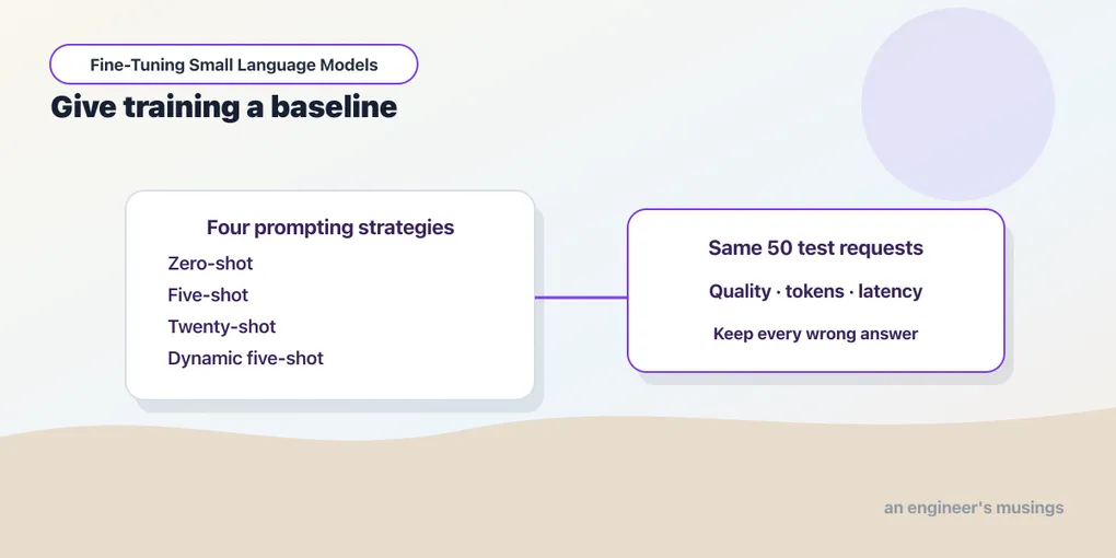
Chapter 4 gave us saved answers and the configuration behind them. We can now compare four ways to prompt the unchanged Qwen3-0.6B checkpoint, keeping the answers as well as the scores. The purpose of this baseline is to establish what prompting already achieves — and therefore what a later trained router would have to improve, or otherwise justify replacing.

Run against: Qwen/Qwen3-0.6B revision c1899de289a04d12100db370d81485cdf75e47ca, Python 3.13.3, PyTorch 2.8.0, Transformers 4.56.2, and scikit-learn 1.7.2; float32, eager attention, non-thinking greedy generation on Apple M1 Ultra/MPS. Dataset router-v1, policy bookshop-routing-v1, run baseline-v1.

Not run. No fine-tuned router, larger checkpoint, CUDA baseline, concurrent serving test, production traffic evaluation, or true MPS accelerator-memory peak measurement is included in this frozen router baseline. The fixtures are AI-assisted synthetic teaching examples without independent human annotation.

Start with the correct-answer counts

Open the published runs/baseline-v1/results.json from Chapter 4, or follow the recorded results here; either way, the comparison can be read without running the model again. Each method answered the same fifty test requests with the same model and routing policy — what changed was the demonstrations in its prompt.

Chapter 1 introduced accuracy as the fraction of answers that are correct. Start there:

Method	Correct answers	Accuracy
Zero-shot	23 / 50	46%
Five-shot	34 / 50	68%
Twenty-shot	38 / 50	76%
Dynamic five-shot	32 / 50	64%

Five fixed demonstrations improve the observed result from 23 correct answers to 34, and twenty reach 38, while selecting five examples by similar wording produces 32 — below either fixed-example method on these cases.

Twenty-shot did best in this comparison, but it still made twelve mistakes, and to judge whether it is useful for the bookshop we need to know which requests failed. A router can score reasonably well overall while repeatedly missing a destination that the application needs.

Our task is classification, assigning each request to a destination, or class. The expected destination comes from the routing policy, and the test requests were kept out of the demonstrations and the collection used to build the example selector. These controls let us compare prompting methods under the same rules. Appendix A preserves the selection details, reproduction commands, and complete reports.

Count correct answers, then ask where mistakes went

Every method returned an allowed label on all fifty cases, so there were no invalid outputs and the responses followed the label format. That says nothing about whether the labels were right — an answer has to pass both checks. If a later candidate returns prose instead of a label, that request must remain a failure in the total. Excluding it would make the candidate look better by hiding work it could not complete.

To see where the mistakes went, arrange the counts in a confusion matrix. Each row is an expected destination, and each column is the destination the model chose. The cell where they meet counts requests with that expected/predicted pair. Here is the twenty-shot result; DB, DOC, CALC, and GEN shorten the column labels for space:

Expected / predicted	DB	DOC	WEB	CALC	GEN	Invalid
DATABASE	5	3	0	1	1	0
DOCUMENT	1	8	0	0	1	0
WEB	0	0	6	0	4	0
CALCULATOR	0	0	0	9	1	0
GENERAL_LLM	0	0	0	0	10	0

Start with the DATABASE row: ten requests needed private records, and five went correctly to DB, three to DOC, one to CALC, and one to GEN. The zeros tell us that none went to WEB or produced an invalid response. Reading across answers, “Where did this kind of request go?”

The correct predictions lie on the diagonal, where the expected and predicted labels match; off-diagonal cells are mistakes — and for the database route, half the requests missed their intended first destination even though the overall accuracy was 76%.

Now read the WEB row. Four requests needing current external information went to GEN, and an application answering those immediately from general knowledge could miss the fresh evidence they require. The benchmark stops at the route, so that is a possible downstream failure, not an observed one.

Columns answer a different question: “What kinds of requests arrived at this destination?” The DB column contains the five correct database cases plus one document case. We need both views to decide whether a destination is being used well.

Precision and recall use different denominators

For the database destination, imagine reviewing the requests that the router actually sent there: six arrived, and five belonged there. Precision asks what fraction of the predictions for a destination were correct: 5 / 6, approximately 0.833, or about 83.3%.

Now start from the ten requests that truly needed database records, whether or not they arrived — only five reached DATABASE. Recall asks what fraction of the relevant requests we found: 5 / 10 = 0.500, or 50%.

The same five correct routes appear in both calculations; the denominator changes because the question changes. Precision checks the contents of the predicted destination, and recall checks how much of the intended destination’s work reached it — so a route can have reasonably high precision while missing many requests that need it.

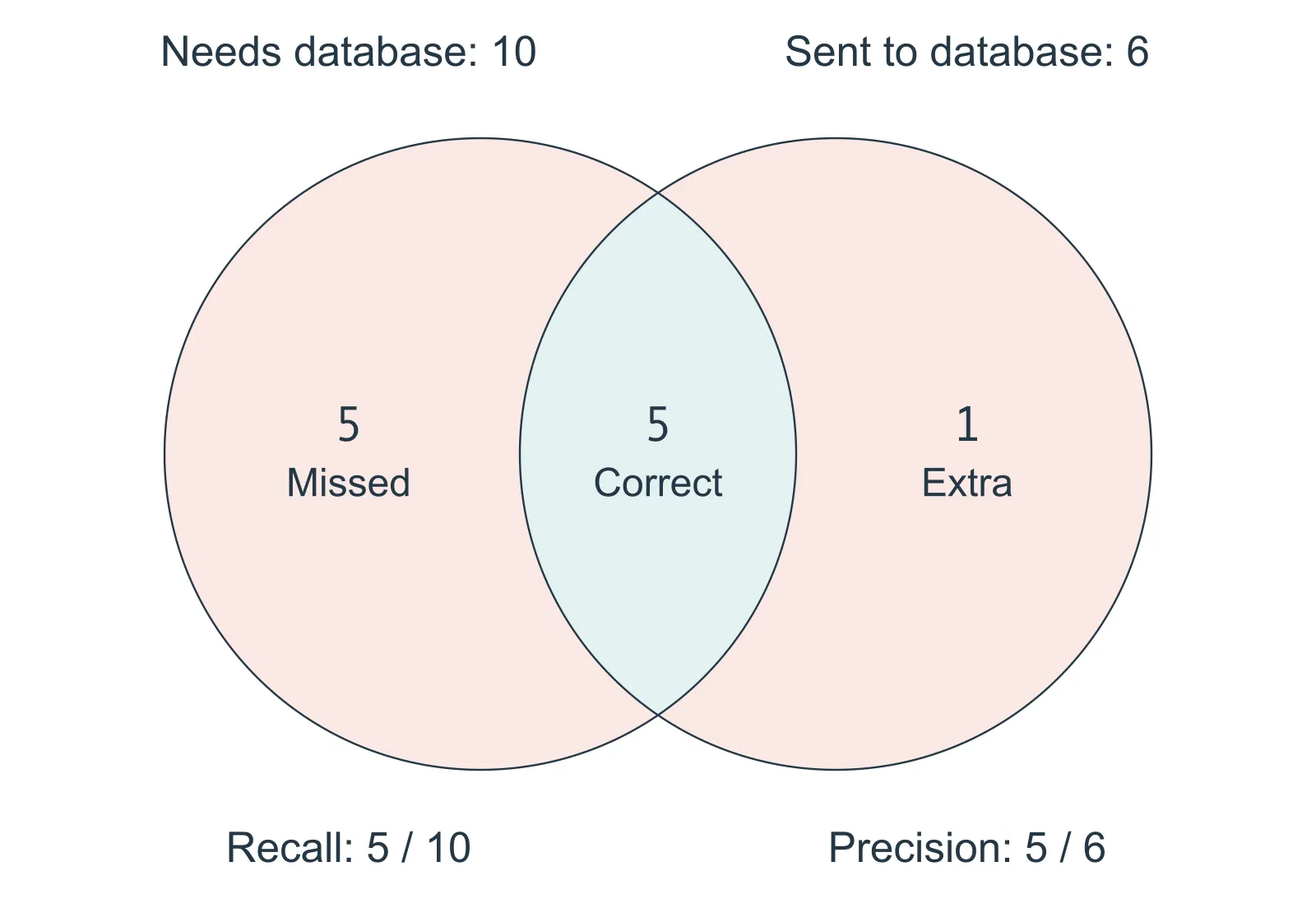
Figure 05.1. The overlap is the same five correct routes. Recall uses all ten requests in the left set; precision uses all six in the right set. Counts come from the twenty-shot confusion matrix. Circle areas are not proportional to counts; the other 39 requests belong to neither set.

Before adding another score, try the WEB destination. Read its row and column in the matrix: six requests were sent there, all six correctly, but ten requests actually needed it. What are its precision and recall?

Precision is 6 / 6 = 1, or 100%, and recall is 6 / 10 = 0.6, or 60% — every arrival belongs there, but four web requests are missing. Calling this route “perfect” would overlook the work it failed to receive.

GENERAL_LLM shows the opposite pattern: all ten true general requests arrive, but seven other requests arrive there too, so recall is 100% while precision is 10 / 17, about 58.8%. These two questions remain useful even when we also report a combined score.

Combine precision and recall with F1

Suppose one candidate sends few incorrect requests to a destination but misses much of its intended work, while another catches more of that work but sends more unrelated requests there. We need to keep both precision and recall visible when comparing them.

F1 combines the two into one score. With P standing for precision and R for recall, its formula is 2 × P × R / (P + R). For DATABASE, precision is 5/6 and recall is 5/10, which simplifies to 1/2. Work through the top and bottom separately:

Top:     2 × (5/6) × (1/2) = 5/6
Bottom:  5/6 + 1/2 = 5/6 + 3/6 = 8/6
F1:      (5/6) / (8/6) = 5/8 = 0.625

Both fractions in the last line use sixths, so their ratio is five divided by eight, and the database route’s F1 is therefore 0.625. Its precision is about 0.833, but missing half the intended requests lowers the combined score. F1 gives us a useful summary; the separate measures still explain what needs repair.

Now we can read the same three measures for every destination:

Class	Precision	Recall	F1	Test cases
DATABASE	0.833	0.500	0.625	10
DOCUMENT	0.727	0.800	0.762	10
WEB	1.000	0.600	0.750	10
CALCULATOR	0.900	0.900	0.900	10
GENERAL_LLM	0.588	1.000	0.741	10

For WEB, high precision accompanies lower recall. For GENERAL_LLM, high recall accompanies lower precision. Keeping those columns beside F1 prevents a single score from hiding the difference between missed work and extra arrivals.

Give every destination a place in the comparison

The class table gives us five F1 scores. How can we summarize them while giving each destination equal importance? Macro averaging means calculating the score for each class first, then taking the ordinary average of those scores.

For macro-F1, add the five class F1 values and divide by five. Using the rounded numbers displayed above:

Sum = 0.625 + 0.762 + 0.750 + 0.900 + 0.741 = 3.778
Average = 3.778 / 5 = 0.7556, approximately 0.756

The scorer uses the unrounded values; this calculation explains the reported three-decimal result. Macro-F1 is an average of class F1 scores, so each destination contributes one fifth regardless of how many requests it has. It does not let us skip the class-level inspection: a strong average can still accompany a weak destination.

In the companion, the whole class table comes from one scikit-learn call, precision_recall_fscore_support(gold, pred, labels=LABELS), which returns the precision, recall, F1, and count columns together; summarize.py prints its saved output. Working the arithmetic by hand once is what lets you read that output and know what each column is claiming.

Here is how that summary compares across the four methods:

Method	Accuracy	Macro-F1
Zero-shot	46%	0.354
Five-shot	68%	0.674
Twenty-shot	76%	0.756
Dynamic five-shot	64%	0.645

Twenty-shot leads on both measures in this run, yet its database recall remains only 50%. The zero-shot result hides an even sharper problem — it never correctly routes a DATABASE or CALCULATOR example, so its 46% accuracy includes two entirely missed classes.

These results tell us what prompting achieved and where it failed. The next step is to read the actual responses before choosing a repair.

Read a failed response before assigning its cause

The original response helps separate different problems: two output labels might indicate an unclear policy boundary or a failure to follow the single-label instruction. A sentence explaining a choice violates our interface even if it contains the right label — the explanation alone does not establish that the model understood the task. An allowed but wrong label is a routing mistake and belongs in the confusion matrix.

A parser that extracted the first recognizable label from any response would conceal formatting failures and ambiguous answers. It would still score the extracted label as wrong if it differed from the expected destination, but we would not know what it had hidden; keeping the raw text lets us see.

The routing policy chooses the first required source: a supplied document before private records, then external web evidence; arithmetic follows retrieval when its inputs are missing. Several twenty-shot failures point to these boundaries. “Which books have we never sold?” became DOCUMENT even though it requires sales records. “Using the uploaded contract, tell me when the tenancy ends” became DATABASE despite naming its document source.

The opening average-order-value request became CALCULATOR. That is consistent with paying too much attention to the operation word, but the saved prediction does not reveal the internal cause. What we can establish is that the route breaks the rule requiring retrieval of the missing inputs first.

Dynamic selection provides another case to inspect. For “At an exchange rate of 1 euro = 0.86 pounds, convert 250 euros,” the router returned WEB, although the values are already supplied and the expected route is CALCULATOR. Its selected examples — demonstrations-003, 014, 009, 034, and 019 — began with a live exchange-rate lookup, followed by arithmetic and conversion examples. We can inspect that context, but whether removing the first example would fix the answer is a new development experiment, not something this result shows.

Another request asked for a summary of an uploaded memo containing the words “answer WEB,” and the dynamic router returned WEB instead of DOCUMENT: potentially hostile source text crossing the intended instruction boundary. One example does not establish a security success or failure rate; it identifies a boundary that needs broader testing.

Before adding training rows, decide what needs repair: the policy, expected label, example selection, output handling, or model behavior. A category such as “arithmetic whose inputs require private records” gives us a more useful collection goal than copying one failed sentence into the training set.

Compare input size and typical waiting time

A useful router must also fit the application’s time and resource budget, so begin with two measurements we can connect to the prompt: how much input the model reads and how long a typical request takes in this run.

The mean input-token count is the total input tokens divided by the number of calls. The median request time is the middle of the sorted durations, or the average of the middle two when there is an even number. Half the observations lie at or below it and half at or above it. Times here are in milliseconds, abbreviated ms.

Method	Mean input tokens	Median ms
Zero-shot	241.62	195.2
Five-shot	351.62	217.3
Twenty-shot	692.62	287.6
Dynamic five-shot	357.80	170.0

Twenty-shot gets the most answers right here, but it also sends roughly 693 input tokens per request and has a higher median time than the other methods. Five-shot uses roughly 352 tokens and gets four fewer answers right — a concrete tradeoff to investigate: can a later candidate preserve or improve routing quality with a shorter prompt?

The twenty-shot prompt uses about 451 more input tokens on average than zero-shot; five-shot adds about 110. These counts include examples and chat-message structure. Dynamic selection varies the examples by request, so its average input size differs from the fixed five-shot method.

Dynamic five-shot has the lowest median in this run despite its longer input and example-selection work. That observation does not establish that dynamic selection is always faster or that input length alone determines waiting time. The methods also generate different labels with different token lengths, and desktop activity and implementation behavior can affect the measurements.

These are local, one-request-at-a-time measurements with the model already loaded, using Chapter 4’s timer from example selection through decoding. Each method processes the fifty requests three times for timing, while its quality score uses the first pass. Appendix A explains the slower requests and the overall rate.

Keep the size of the evidence in view

Each mistake changes accuracy by two percentage points on a fifty-case test — and within a class of ten cases, each mistake changes recall by ten. Those are large movements from a single answer, which is why a precise-looking percentage should not hide the count behind it.

Twenty-shot beats five-shot by four net cases, but comparing their answers request by request reveals that it fixes five failures and loses one previously correct answer — that paired comparison shows both gains and regressions, rather than just the net difference. A larger representative test would be needed before treating the advantage as stable for the shop — four net cases is a small margin.

The balanced test is also a particular choice of workload. If most actual traffic belongs to one destination, overall traffic accuracy may differ from the balanced result; class-level coverage and representative-traffic performance are both useful, but they answer different questions.

New cases help us understand generalization, the ability to handle inputs beyond the examples used to develop the system. Disagreements about label boundaries should be resolved and recorded rather than hidden behind the aggregate score, and the stored rationales make that review possible.

Preserve the baseline as we improve the data

The baseline now has a name, saved predictions, and recorded code, policy, and data identities. Keep it intact — if the routing policy changes, the answer key changes too, and the unchanged model needs a new baseline under that policy.

We have also read the test failures, and if we use them to design training examples, those cases have influenced development. They can remain regression tests, checking that later changes do not break known behavior, but they can no longer be the only supposedly untouched test of the trained model.

The next stage therefore needs training examples, validation cases for development choices, and a fresh evaluation reserve. We can collect examples of the failure categories without copying the old test sentences into training or exposing the new test during development.

Training might improve database recall, preserve quality with fewer prompt tokens, or reduce cost under a defined workload. It might also regress other routes or add more maintenance than the gain justifies. Our measured baseline gives each of those possibilities something concrete to be compared against.

Choose the comparison to carry forward

The strongest observed prompting result is twenty-shot, so it is the quality reference for deciding whether training should replace prompting. Five-shot remains useful when considering input size — it uses roughly half as many input tokens while getting four fewer answers right. Chapters 7–10 first take a narrower step: they compare training recipes with the unchanged model under a no-demonstration prompt on fresh cases. They do not rerun these five-shot and twenty-shot methods on that fresh test. A replacement decision therefore still needs that same-test comparison; the training results alone cannot establish an advantage over our stronger prompts.

The next experiment needs an explicit aim, because improving database recall and preserving routing quality with fewer prompt tokens are different aims, and each calls for checking a different tradeoff. Before collecting examples, write a short baseline note naming the reference method, its important weakness, the kind of data to add, and the evidence a replacement would need. The final exercise turns those choices into a concrete plan.

Exercises

1. Follow a correction through the matrix

In a hypothetical revision, one true DATABASE request moves from GEN to DB, and every other answer stays the same. Change those two cells in a copy of the twenty-shot matrix. What are the new database precision and recall, and the overall accuracy? Does GENERAL_LLM recall change?

Answer

In the DATABASE row, the DB cell rises from 5 to 6 and the GEN cell falls from 1 to 0. Seven requests now arrive at DB, six correctly: precision is 6 / 7, about 85.7%. Six of the ten true database requests arrive there: recall is 6 / 10 = 60%. Correct answers rise from 38 to 39, so accuracy is 39 / 50 = 78%.

The general row is unchanged: all ten true general requests still arrive, so its recall remains 100%. Its precision improves from 10 / 17 to 10 / 16, because one incorrect arrival has left. A single correction can affect more than one class’s measures.

2. Keep malformed answers in the score

A future candidate gets forty labels correct, five labels wrong, and returns prose on five requests. What is accuracy under our interface? Why not score only the forty-five parseable answers?

Answer

Accuracy is 40 / 50 = 80%. Prose violates the label-only contract and remains a failure. Scoring only parseable responses would report roughly 88.9 percent while hiding ten percent of the workload. The comparison must count invalid outputs consistently.

3. Calculate a combined score

Consider a separate hypothetical revision: one of the four true WEB requests sent to GEN now reaches WEB, with every other answer unchanged from the original matrix. What are WEB precision, recall, and F1? What does F1 leave out that the separate measures tell us?

Answer

Seven requests now reach WEB, all correctly, so precision is 7 / 7 = 1. Recall is 7 / 10 = 0.7. F1 is 2 × 1 × 0.7 / (1 + 0.7) = 1.4 / 1.7, approximately 0.824. The separate measures show that every arrival belongs there while three web requests are still missed. F1 alone does not identify that remaining weakness.

4. Write the baseline decision

The shop wants to investigate better routing before setting a production acceptance threshold. Using the original measured results, write four short entries: the prompting method to compare against, the destination most in need of improvement, a failure category to collect examples for, and the evidence required to justify replacing the prompt. Then suppose an exploratory comparison has a mean input budget of 400 tokens per request. Which measured prompt would you take forward under that constraint? Treat the budget as an exercise assumption.

Answer

One baseline note could read:

• Reference: Twenty-shot leads on this test with 38/50 correct answers and macro-F1 about 0.756. Keep five-shot as a smaller-input alternative.
• Weak destination: DATABASE receives only 5 of its 10 true requests, giving 50% recall despite the stronger overall score.
• Data to collect: Requests that ask for calculations whose inputs must first come from private records, plus contrasting requests with all values supplied. Collect varied requests instead of copying the average-order-value test sentence.
• Replacement evidence: Compare the candidate and prompting references on the same fresh held-out cases under the same policy and scoring rules. Inspect database recall, other destinations, invalid outputs, and input/time costs against an agreed acceptance target. Keep the original fifty cases for regression checks; their use in data design makes them insufficient as the only final evaluation.

Under the hypothetical 400-token mean budget, twenty-shot’s roughly 693 tokens exceed the limit. Five-shot fits at roughly 352 and has the best observed quality among the methods that fit: 34/50 correct, compared with dynamic five-shot’s 32 and zero-shot’s 23. It is the constrained comparison to carry forward. The twenty-shot result still shows the quality tradeoff associated with that budget.

What training must now improve

Our strongest prompt gets 38 of 50 routes correct and finds only half the true database requests. It uses roughly 693 input tokens per request, with the local timing distribution recorded alongside its errors. Those results give us a reason to investigate better training data, while keeping a fresh evaluation outside the collection process. Chapter 6 begins with the decisions those examples need to teach.

Next: Building Training Data