Stop Paying the Flattening Tax

Almost all the data anyone hands you is nested. An API response has objects inside objects. A log line has an array of tags. An order has line items. That is the natural shape.

A relational table is flat, so something has to give, and there are only two conventional answers. Store the nested part as a JSON string and lose every type inside it. Or normalise it into a side table and pay for a join every time you want it back.

Both are real costs, and both are so familiar that we stopped calling them costs. Call it the flattening tax: you pay it on the way in, and you pay it again on every query.

DuckDB does not charge it. Lists, structs and maps are first-class types with their own storage, their own functions, and no penalty for using them. This chapter is about what that changes, and about the small number of places where the semantics will surprise you.

Everything here was run against DuckDB 1.5.5 on the book’s edge-log dataset.

Three types, three jobs

select typeof([1, 2, 3]);
select typeof({'a': 1, 'b': 'x'});
select typeof(map([1, 2], ['a', 'b']));

INTEGER[]
STRUCT(a INTEGER, b VARCHAR)
MAP(INTEGER, VARCHAR)

Look at what the type strings contain, because that is the whole design.

A LIST is ordered and homogeneous. INTEGER[] says integers, any number of them. The element type is part of the type, so a mixed list is not a thing:

select [1, 'x'];

Conversion Error: Could not convert string 'x' to INT32

A STRUCT carries its field names and their types in the type itself. STRUCT(a INTEGER, b VARCHAR) is a different type from STRUCT(b INTEGER). The shape is fixed and known at plan time.

A MAP has one key type and one value type, and any number of entries. The keys are data, not schema.

They compose without limit:

select typeof([{'a': [1, 2]}]);

STRUCT(a INTEGER[])[]

A list of structs, each holding a list. That is an ordinary type, and every operation below works on it.

Struct or map: decide by the failure

Both look like “a thing with named parts”, so the choice feels arbitrary until you see them fail. Ask each for something that is not there.

A struct:

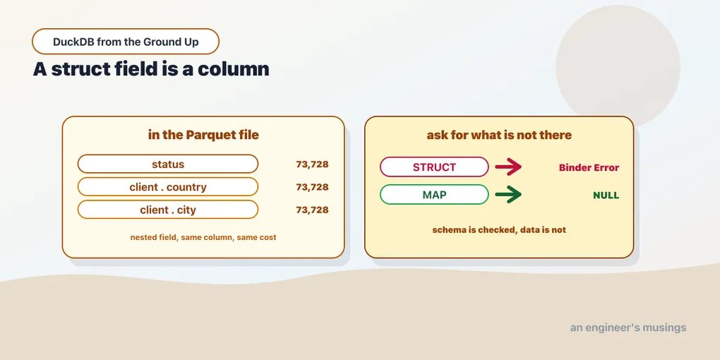
select ({'a': 1}).zzz;

Binder Error: Could not find key "zzz" in struct

A map:

select map([1, 2], ['a', 'b'])[9];

NULL

The struct raised a binder error. The map returned NULL.

That is not a quirk, it is the distinction stated precisely. A struct’s fields are schema: they are in the type, so DuckDB checks them while planning, before a single row is read. A typo fails immediately and fails the same way every time. A map’s keys are data: nothing can be checked in advance, so a missing key is an absent value like any other.

Which gives a rule you can apply without thinking about it:

Use a STRUCT when the field names are part of your design. A client with country and city. An address. A geo point. You know the fields, you want a typo caught at plan time, and you want each field to have its own type.

Use a MAP when the keys come from the data. User-supplied attributes, per-tenant custom fields, HTTP headers, anything where a new key appearing is normal rather than a schema change.

The failure modes are the tell. If “that key wasn’t there” should be an error, you want a struct. If it should be a NULL, you want a map.

The indexing trap

Lists are 1-based:

select [10, 20, 30][1];

10

Fine, if surprising for anyone arriving from Python. The trap is the next one:

select [10, 20, 30][0];

NULL

Index 0 is not an error. It is a silent NULL, in a language where indexing starts at 1. Every Python habit you have says [0] is the first element, and here it is nothing at all. No warning, no exception — just a null that flows downstream and turns an aggregate into a slightly wrong number.

This is the single most likely way to write a quietly incorrect query with nested data. Give it a moment of deliberate attention every time you index a list by a literal.

Out-of-range behaves the same way:

select [10, 20, 30][9];

NULL

Negative indexing does work, from the end:

select [10, 20, 30][-1];    -- 30
select [10, 20, 30, 40][2:3];   -- [20, 30]

So the mental model is: 1-based, forgiving, and never an error. Which is convenient right up until it is not.

The real data

The edge logs carry both a struct and a list:

select tags, client from 'edge/**/*.parquet' limit 2;

(['edge'],                        {'country': 'US', 'city': 'NYC'})
(['edge', 'cache-hit', 'beta'],   {'country': 'US', 'city': 'NYC'})

Struct fields are ordinary expressions. Group by one:

select client.country, count(*) from 'edge/**/*.parquet'
group by 1 order by 2 desc, 1 limit 2;

('BR', 100000)
('DE', 100000)

Lists need unnest, which turns one row with a three-element list into three rows. There is one wrinkle worth knowing before you hit it:

select unnest(tags) tg, count(*) from 'edge/**/*.parquet' group by 1;

Binder Error: UNNEST not supported here

unnest produces rows, so it cannot sit in a query that is also grouping — the expansion has to happen first. Put it in a subquery:

select tg, count(*) from (select unnest(tags) tg from 'edge/**/*.parquet')
group by 1 order by 2 desc;

('edge',      500000)
('cache-hit', 333333)
('beta',      166666)

Every row has edge, two thirds have cache-hit, one third has beta. That is a tag-frequency report over half a million rows, from data nobody flattened, in one query with no join.

unnest on a struct does something different and equally useful — it expands the fields into columns:

select unnest(client) from 'edge/**/*.parquet' limit 2;

('US', 'NYC')
('US', 'NYC')

And recursive := true goes all the way down:

select unnest({'a': 1, 'b': {'c': 2}}, recursive := true);

(1, 2)

Lists have a functional standard library

The part that stops nested data being awkward is that lists come with the operations you would otherwise write a loop for:

select list_transform([1, 2, 3], x -> x * 10);     -- [10, 20, 30]
select list_filter([1, 2, 3, 4], x -> x % 2 = 0);  -- [2, 4]
select list_reduce([1, 2, 3, 4], (a, b) -> a + b); -- 10
select list_sort([3, 1, 2]);                        -- [1, 2, 3]

Map, filter and reduce with lambda syntax, inside SQL, on a column. This is where nested types stop being a storage detail and start being a way to express things. A per-row transformation over an array does not need a unnest, a computation and a re-aggregation. It is one function call, and it stays inside the vectorized engine — which chapter 7 argued is the thing that matters most.

Going the other way, list() is an aggregate that collects rows into a list:

select list(i) from range(4) t(i);

[0, 1, 2, 3]

So unnest and list() are inverses, and you can drop into flat-row-land for one step and come back. There are matching builders for the other types — struct_pack(a := 1, b := 'x'), struct_insert({'a':1}, b := 2), map_from_entries, map_keys, list_zip — and to_json / from_json to cross between nested types and JSON text.

What it costs: nothing

The reasonable suspicion is that all this convenience is paid for at scan time. It is not:

struct field group by  :  2.2 ms
plain column group by  :  2.0 ms

Grouping by client.country costs essentially what grouping by status costs, and the reason is in the file layout:

select path_in_schema, type, num_values
from parquet_metadata('edge/dt=2026-03-01/data_0.parquet');

('status',           'INT32',      73728)
('client, country',  'BYTE_ARRAY', 73728)
('client, city',     'BYTE_ARRAY', 73728)
('tags, list, element', 'BYTE_ARRAY', 147456)

client.country is its own physical column, sitting beside status with exactly the same number of values. The struct is not a blob that gets parsed per row. It is a naming convention over columns that are stored separately — which is why the projection pushdown from chapter 7 could read client.country and leave client.city on disk.

Lists cost slightly more, and the numbers say why: 147,456 values for tags against 73,728 rows, because the list elements are stored flat with separate length information. Reading a list means reconstructing rows from that, and the len(tags) group-by measured 4.5 ms against 2.0 for a plain column. Twice as much for a variable-length type, which is the honest price and a long way from a JSON parse.

When to flatten anyway

Nested types are not always the answer, and three cases are worth naming.

When the consumer cannot take them. A BI tool, a CSV export, an ancient JDBC client — all flat. Chapter 4 already showed that writing nested columns to CSV loses them entirely. Keep the data nested and flatten in a view at the boundary, rather than flattening at rest.

When the list is really a table. A list of a handful of tags is a value. A list of ten thousand line items, each needing its own filters and joins, is a table that has been folded into a column. The tell is whether you find yourself unnesting it in most queries — if so, it wants to be rows.

When the shape is genuinely unknown. A struct is a schema, and a schema you cannot write down is not a schema. That case has its own answer, which is the next chapter.

Final thoughts

The flattening tax is easy to miss because it is charged in habits rather than in milliseconds. You destructure the API response before you store it. You write the join. You reach for a JSON string and accept that everything inside it is text now. None of that felt like a decision.

DuckDB’s three nested types make it a decision, and the measurements say the default should flip: a struct field is a real column and costs what a real column costs. The nesting is free, and the type information you would have thrown away is still there.

Two things to keep. Choose struct versus map by which failure you want — a binder error for a typo, or a NULL for a missing key. And list[0] is NULL, not the first element, in a language that starts at 1 and never raises an index error. The first is a design principle. The second will cost someone a day.

Next: The Shape You Cannot Write Down — VARIANT, JSON, and what to do when the schema is genuinely not knowable in advance.