Streaming Facts: When the Nightly Batch Stops Being Nightly
Micro-batching, hot/cold splits, Snowflake Streams, Tasks, and Dynamic Tables — how a star schema survives minute-level latency, exactly what breaks dimensionally when it does, and the honest test for whether you need any of it.
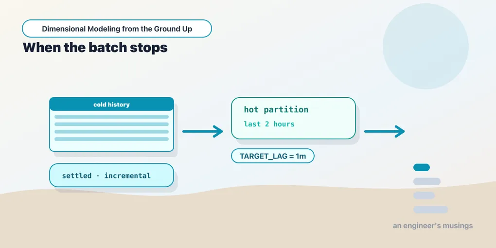
Every model in this book has quietly assumed that the warehouse gets to think overnight.
The facts rebuild at 2 a.m. The snapshots run once a day. The aggregate reprocesses its lookback while nobody is looking, and by the time an analyst opens a dashboard, everything agrees with everything else. That assumption is load-bearing in ways you may not have noticed. It’s why dbt snapshots can get away with dating a change to when they observed it. It’s why a merge on a hundred-million-row fact is fine — you do it once. It’s why “as of when?” has never come up, because the answer was always “last night, same as everything else on this page.”
Then someone asks for the sales dashboard to be live. Not “refreshed by 8 a.m.” — live.
This chapter is what happens to a dimensional model when latency drops from a day to minutes: which of your patterns were secretly latency-dependent, and which weren’t. One of them — the deterministic surrogate key — turns out to be the reason streaming is possible at all. Two others — the periodic snapshot, the scheduled Type 2 snapshot — turn out to be definitionally batch. We’ll build it three ways on the bookshop, then spend the last section on when not to, because this is the chapter where people most reliably set money on fire.
What batch was quietly assuming
Three things break, in order.
The quiet period. A batch star has a window where nothing arrives, so models build in dependency order and are consistent when they finish: dim_customer is built, then fct_order_items resolves keys against it, then the aggregate rolls up the fact. Every layer sees a settled version of the layer beneath it. Delete the quiet period and that’s gone — the fact is written while the aggregate reads it, and consistency becomes something you design for rather than something the clock hands you.
“As of when?” In batch, every table has the same answer, so nobody asks. Streaming, the fact might be 40 seconds behind the source, dim_customer 20 minutes behind, and the daily aggregate 6 hours behind — and a query joining all three returns a number that is as of an incoherent mixture of three moments. It won’t look wrong. It’ll be quietly unattributable, because the discrepancy is time and time isn’t a column in the result. Every streaming fact needs an ingestion audit column, and every consumer needs a way to ask how fresh the thing in front of them is.
The merge cost curve. This one shows up on the bill. Snowflake stores data in immutable micro-partitions; any DML touching a row rewrites the whole partition, and a MERGE must first scan the target to find its matches — all of it, if nothing lets it prune. Do the arithmetic, because nobody does it in advance. fct_order_items is 400 GB; your nightly merge scans it once. Run that merge every minute and it’s 1,440 runs a day, each scanning 400 GB: 576 TB of reads per day to apply maybe fifty thousand rows. Batch hides this because you pay the scan once. Frequency turns a fixed cost into a per-run cost, and per-run costs multiply.
Consistency, provenance, and a cost curve pointing the wrong way. Everything below answers one of those three.
Micro-batching: shrink the interval, not the architecture
The honest first answer to “we need it faster” is almost never “we need a streaming architecture.” It’s “run what you already have, more often.” A dbt model on a fifteen-minute schedule is real-time enough for the overwhelming majority of what gets called real-time, and it adds no new failure modes. Start here; earn your way to anything else.
But shrinking the interval doesn’t shrink the problems proportionally — it sharpens one.
Event time versus ingestion time
Late-arriving data was a chapter about days: a correction lands three weeks after the order. At a fifteen-minute cadence you meet the identical problem at the scale of seconds, and it stops being an edge case and becomes every run.
The standard watermark is where event_ts > (select max(event_ts) from {{ this }}). It works nightly because by 2 a.m. nothing from yesterday is still in flight. It fails at fifteen minutes because something is always in flight: an order committed at 10:14:59 lands in staging at 10:15:03, by which time the 10:15:00 run has taken max(event_ts) = 10:14:58 and moved on. That order is now permanently behind the watermark. It will never be selected again, and nothing errors.
The fix is to stop conflating two timestamps that batch let you treat as one. Event time (order_ts) is when the business thing happened — it’s what the model means, and it is not monotonic, because events arrive out of order. Ingestion time (_ingested_at) is when the row landed in your table, stamped by the loader — and it is monotonic, because you control it. So: watermark on ingestion time; filter, partition, and report on event time. A late event has a low event_ts but a high _ingested_at, so an ingestion-time watermark catches it however late it is. One column, and an entire class of silently-dropped-row bugs disappears.
-- models/marts/fct_order_items.sql
{{ config(
    materialized='incremental',
    unique_key='order_item_sk',
    incremental_strategy='merge',
    cluster_by=['order_date'],
    incremental_predicates=[
        "DBT_INTERNAL_DEST.order_date >= dateadd(day, -3, current_date)"
    ]
) }}

with source_rows as (

    select * from {{ ref('stg_order_items') }}

    {% if is_incremental() %}
    where _ingested_at > (select max(_ingested_at) from {{ this }})
    {% endif %}

)

select
    {{ dbt_utils.generate_surrogate_key(['order_id', 'line_number']) }} as order_item_sk,

    {{ dbt_utils.generate_surrogate_key(['book_id']) }}                     as book_sk,
    {{ dbt_utils.generate_surrogate_key(["coalesce(customer_id, '-1')"]) }} as customer_sk,
    {{ dbt_utils.generate_surrogate_key(['order_date']) }}                  as date_sk,

    order_id, order_date, order_ts,
    quantity, extended_price, _ingested_at

from source_rows
qualify row_number() over (
    partition by order_id, line_number
    order by _ingested_at desc
) = 1
Three things in there are doing streaming work.
The qualify is not optional. Streaming delivery is at-least-once: Kafka replays, loaders retry, a Snowflake stream hands you two versions of a row that changed twice in one window. A MERGE given two source rows for one target key fails outright — Duplicate row detected during DML action — so collapsing each natural key to its latest version before the merge sees it is the difference between a pipeline that works and one that works until the first retry.
incremental_predicates bounds the merge’s target scan. Those predicates go into the on clause of the generated MERGE, against the target alias DBT_INTERNAL_DEST — so instead of scanning 400 GB for matches, Snowflake prunes to three days of partitions. With cluster_by=['order_date'] co-locating rows by date so the pruning actually prunes, this is what flattens the cost curve above.
And it comes with a knife. Bounding the target means the merge cannot see rows outside the bound. An order line corrected six days late won’t match its existing row, so the not matched branch fires and you get a duplicate, not an update. A predicate you added for cost has silently become a correctness constraint. Set it to your real correction horizon, not to whatever makes the query fast, and keep the uniqueness test from the testing chapter on order_item_sk so the day the horizon is wrong, the build goes red instead of the number going wrong.
The microbatch strategy
dbt 1.9 added an incremental strategy built for this shape. Declare the event-time column and a batch size, and dbt splits the run into independent, time-bounded batches, each replacing its own window in the target:
{{ config(
    materialized='incremental',
    incremental_strategy='microbatch',
    event_time='order_ts',
    batch_size='hour',
    lookback=3,
    begin='2026-01-01'
) }}
Note what’s gone: no is_incremental(), no watermark. dbt applies the time filter itself, because you told it which column carries event time. lookback=3 says “also reprocess the three hourly batches before the current one” — the late-arrival window, declared as config rather than buried in a where clause. Each batch is idempotent, so a backfill stops being a scary --full-refresh: dbt run --select fct_order_items --event-time-start "2026-07-01" --event-time-end "2026-07-08". (The upstream model or source must also declare event_time, so dbt knows what to filter it on.)
The trade is that microbatch is window-shaped — it replaces time windows — which makes it a natural fit for an append-only transaction fact and a poor one for an accumulating snapshot whose rows update forever. Hold onto that; the fact type is about to tell you a great deal.
The hot/cold split
Micro-batching gets you to minutes. Below that the merge is the wrong instrument: you’re paying partition-rewrite costs to maintain a table whose recent tail churns constantly and whose deep history hasn’t moved in months. Those regions want different physics.
So split them. A cold table holds settled history, maintained incrementally at whatever cadence you like. A hot relation is a view over the landing table covering the last few minutes — nothing to rebuild, because there’s almost nothing in it. The fact everyone queries is a view unioning the two.
The one critical decision is where to cut, and there’s exactly one right answer: cut on ingestion time, not event time. Cut on event time and out-of-order arrivals fall down the crack — an order with order_ts = 09:58 that lands at 10:07 is below the cold table’s event-time cutoff and arrived after its last build, so it exists in neither half. Cut on ingestion time, which is monotonic by construction, and the halves partition the data perfectly however scrambled event time is.
Take the select list from the model above — key hashes, the '-1' routing, measures, the dedupe qualify — and lift it verbatim into macros/order_item_projection.sql, taking the source CTE’s name as its one argument. Then both halves are three lines each:
-- models/marts/fct_order_items_cold.sql — settled history
{{ config(
    materialized='incremental', unique_key='order_item_sk', incremental_strategy='merge',
    cluster_by=['order_date'],
    incremental_predicates=["DBT_INTERNAL_DEST.order_date >= dateadd(day, -3, current_date)"]
) }}

with source_rows as (
    select * from {{ ref('stg_order_items') }}
    where _ingested_at <= dateadd('minute', -{{ var('hot_window_minutes', 30) }}, current_timestamp())
    {% if is_incremental() %}
      and _ingested_at > (select max(_ingested_at) from {{ this }})
    {% endif %}
)
{{ order_item_projection('source_rows') }}
-- models/marts/fct_order_items_hot.sql — whatever the cold table hasn't taken
{{ config(materialized='view') }}
with source_rows as (
select * from {{ ref('stg_order_items') }}
where _ingested_at > (
select coalesce(max(_ingested_at), '1900-01-01'::timestamp_ntz)
from {{ ref('fct_order_items_cold') }}
)
)
{{ order_item_projection('source_rows') }}-- models/marts/fct_order_items.sql — the only thing anyone queries
{{ config(materialized='view') }}
select * from {{ ref('fct_order_items_cold') }}
union all
select * from {{ ref('fct_order_items_hot') }}The hot view derives its boundary from the cold table itself, so the seam is self-healing: if the cold build is late, the hot view covers more; when it runs, the hot view instantly covers less. There’s no window to keep in sync between two models, which means no window to get wrong. The cold table’s <= now - 30 minutes filter merely stops it chasing the tail — an efficiency choice, not a correctness one, and the union stays gapless either way.
Two honest caveats, because this pattern gets sold as free.
Two code paths, one truth. The macro is why the projection can’t drift; without it, hot revenue and cold revenue quietly compute different things and the discontinuity lands exactly at the seam, the last place anyone looks. But a shared macro reduces two code paths to one definition, and that’s as far as the reduction goes: you still have two materializations, two ways to fail, and a union view every dashboard now depends on. So reconcile the halves the way chapter 15 reconciled aggregates against atomic facts — a singular test asserting they’re disjoint costs thirty seconds and catches the only failure that really hurts:
-- tests/assert_hot_cold_disjoint.sql
select order_item_sk from {{ ref('fct_order_items_cold') }}
where order_item_sk in (select order_item_sk from {{ ref('fct_order_items_hot') }})
The hot half is unclustered by design. Fine when it’s thirty minutes of orders. Less fine when the cold build fails at midnight and nobody notices until nine, at which point “the last thirty minutes” is nine hours of unpruned scanning on every query. That’s a slow answer rather than a wrong one — forgiving, as failures go — but you still want the alert.
Letting Snowflake do it: Streams and Tasks
Everything above runs dbt on a clock. Snowflake will run the clock for you, with two primitives from the programmability chapter of the Snowflake series.
A Stream on the landing table is CDC with no triggers and no watermark column: it exposes the rows that arrived since the last consumer, and the offset advances atomically with the DML that consumes it — so reading changes and acknowledging them are one transaction, and a task that dies halfway loses nothing. A Task is a scheduler inside the account; gate it on SYSTEM$STREAM_HAS_DATA and it burns compute only when there’s work.
CREATE OR REPLACE STREAM raw.order_items_stream
  ON TABLE raw.order_items_landing
  APPEND_ONLY = TRUE;

CREATE OR REPLACE TASK analytics.load_fct_order_items
  WAREHOUSE = transform_wh
  SCHEDULE  = '1 MINUTE'
  WHEN SYSTEM$STREAM_HAS_DATA('raw.order_items_stream')
AS
MERGE INTO analytics.fct_order_items AS tgt
USING (
    SELECT
        MD5(COALESCE(CAST(order_id    AS VARCHAR), '_dbt_utils_surrogate_key_null_') || '-' ||
            COALESCE(CAST(line_number AS VARCHAR), '_dbt_utils_surrogate_key_null_')) AS order_item_sk,
        MD5(COALESCE(CAST(customer_id AS VARCHAR), '-1'))                             AS customer_sk,
        -- ... book_sk, date_sk, measures, CURRENT_TIMESTAMP() AS _ingested_at
        order_id, order_date, order_ts, quantity, extended_price
    FROM raw.order_items_stream
    QUALIFY ROW_NUMBER() OVER (
        PARTITION BY order_id, line_number ORDER BY order_ts DESC) = 1
) AS src
ON  tgt.order_item_sk = src.order_item_sk
AND tgt.order_date   >= DATEADD(day, -3, CURRENT_DATE)      -- prune the target
WHEN MATCHED     THEN UPDATE SET tgt.quantity = src.quantity, ...
WHEN NOT MATCHED THEN INSERT (...) VALUES (...);

ALTER TASK analytics.load_fct_order_items RESUME;
Stare at those MD5 expressions, because they’re the most dangerous lines in the chapter. dbt_utils.generate_surrogate_key is not magic: it compiles to md5 of each field cast to varchar, null-coalesced to the literal _dbt_utils_surrogate_key_null_, joined with -. Hand-write a merge that hashes slightly differently — another separator, another sentinel, sha2 instead of md5 — and the streaming path and the dbt path mint different surrogate keys for the same row. Every fact the task loads then fails to join to any dimension dbt built. The joins won’t error; they’ll return nothing, or collapse into the unknown member, and you’ll lose an afternoon. The key expression must live in exactly one place. Generate the task’s SQL from the same macro — or don’t hand-write the task at all, which is a fine argument for the next section.
Three smaller points. APPEND_ONLY = TRUE suits a landing table that only grows and is cheaper than a standard stream; use a standard stream only if downstream must mirror deletes. The AND tgt.order_date >= ... in the ON clause is hand-rolled incremental_predicates — same prune, same knife, same duplicate on a six-day-late correction. And '1 MINUTE' is the floor: Snowflake won’t schedule a task more often, so if you need sub-minute you don’t want a task, you want the ingestion layer writing the fact directly.
Dynamic tables: declare the freshness, delete the plumbing
Streams and tasks work, and they’re also a hundred lines of hand-written merge you now own forever. Dynamic tables are the declarative answer: write the SELECT that defines what the table is, plus a TARGET_LAG saying how stale it may get, and Snowflake works out the refresh — incrementally where the query allows, by full rebuild where it doesn’t. No stream, no task, no merge, no offset. And dbt-snowflake ships it as a materialization, so it belongs in your project rather than a migration script:
-- models/marts/fct_order_items.sql
{{ config(
    materialized='dynamic_table',
    snowflake_warehouse='transform_wh',
    target_lag='5 minutes',
    refresh_mode='AUTO',
    initialize='ON_CREATE',
    on_configuration_change='apply'
) }}

with source_rows as (
    select * from {{ ref('stg_order_items') }}
)
{{ order_item_projection('source_rows') }}
Same macro, same ref, same tests in the same YAML. What’s gone is is_incremental(), the watermark, the merge strategy, the dedupe dance, and the hot/cold union — all collapsed into two config lines. dbt run now declares the table instead of loading it. For most streaming facts, this is the one I’d reach for first.
Now the parts the marketing page doesn’t lead with.
Non-deterministic functions kill incremental refresh. Snowflake can only refresh incrementally if it can reason about how a change to the source changes the result, and it cannot reason through CURRENT_DATE(), CURRENT_TIMESTAMP(), or RANDOM(), which answer differently on every refresh. Which means the most reflexive line in all of incremental modeling — where order_date >= current_date - 3 — is precisely what demotes your dynamic table to a full rebuild every five minutes. That’s the habit to unlearn. The lookback window existed to make an incremental load cheap; the dynamic table is doing that job for you, and the current_date filter is sabotaging it. Write the query as the complete definition of the table and let Snowflake compute the delta.
Verify the refresh mode; never assume it. REFRESH_MODE = AUTO lets Snowflake choose, and it will quietly choose FULL if something blocks the incremental path — and a full-refresh dynamic table on a five-minute lag is 288 complete rebuilds of your fact table per day. So check, every time:
SHOW DYNAMIC TABLES LIKE 'FCT_ORDER_ITEMS' IN SCHEMA analytics;
-- read the refresh_mode and refresh_mode_reason columns

SELECT name, state, refresh_action, refresh_start_time
FROM TABLE(information_schema.dynamic_table_refresh_history())
ORDER BY refresh_start_time DESC LIMIT 20;
refresh_mode_reason names, in words, the construct that disqualified incremental refresh. Declaring REFRESH_MODE = INCREMENTAL explicitly is the paranoid move: an unsupported query then fails at create time rather than silently costing you 288 rebuilds a day. Fail loudly at deploy, not quietly on the invoice.
They chain, and lag propagates. A dynamic table can read another, so a whole staging-to-marts DAG can be dynamic tables end to end. Set the intermediate ones to TARGET_LAG = DOWNSTREAM and they refresh only as often as whatever depends on them needs — freshness flows backward through the graph and you declare it in exactly one place, on the mart the business cares about. It’s the closest the modern warehouse gets to a freshness SLO written as code.
The lag is a cost dial. A dynamic table refreshes on the warehouse you name it, and a one-minute TARGET_LAG means that warehouse essentially never suspends. An X-Small burns a credit per hour it’s awake; awake around the clock is roughly 720 credits a month, landing in the low four figures depending on edition and cloud. Move the same table to an hourly lag and the warehouse might be awake twenty minutes a day. Freshness isn’t a boolean, it’s a slider with a price printed on it — and far fewer dashboards need the one-minute end than there are people who’ll ask for it.
The landing zone: Snowpipe and Snowpipe Streaming
None of this matters if data reaches the warehouse hourly, because a fact is exactly as fresh as its slowest upstream hop.
Snowpipe ingests files as they land in a stage — serverless, event-driven, typically within a minute of the file appearing. Right when your producers already write files. The trap is file size: Snowpipe carries a per-file overhead (on the order of 0.06 credits per thousand files, on top of the compute to load them), so a producer writing a 2 KB file every second will out-earn your entire transform budget in overhead alone. Snowpipe Streaming instead ingests rows, over an API, with no files in the middle — the Kafka connector uses it, as does anything writing through the Snowflake ingest SDK. Latency is seconds, and it’s what makes a one-minute dynamic table meaningful rather than decorative.
The composition is the one the Snowflake series drew: Snowpipe or Snowpipe Streaming lands raw rows; a dynamic table (or a stream and a task) shapes them into the star. Ingestion and transformation stay in separate lanes, and the dimensional model lives entirely in the second one — which is why the previous fifteen chapters still apply.
What actually breaks dimensionally
Push a star to minute latency and four dimensional things change: one for the better, three for the worse.
The surrogate key is why any of this works
Look again at the streaming loader. It computes book_sk, customer_sk, and date_sk without touching a single dimension table. No join, no lookup, no sequence, no key cache — it hashes the natural keys straight out of the payload. That isn’t a convenience. It’s the reason a star schema can be loaded at stream speed at all.
The classical Kimball load does a key lookup: join the incoming fact to dim_customer to fetch the integer customer_key, and if there’s no match, insert an inferred member and take its new key. That’s a join and a possible write against a dimension, per event, in the hot path — and a serializing one, since two concurrent loads meeting the same new customer must not mint two keys for them. At nightly volumes, fine. At ten thousand events a second it’s a distributed-systems problem, and it’s why a generation of streaming warehouses gave up and went denormalized.
Deterministic hashing deletes the problem. hash('8812') is hash('8812') on every node, in every process, at every moment, with no coordination and no state — the fact and the dimension agree on the surrogate key without ever having met, exactly as chapter 10 put it. Nothing to look up, so nothing to serialize, so the fact loader has no dependency on the dimension pipeline at all. And there’s a second dividend: streaming delivery is at-least-once, so the same order line will arrive twice — but its key is a pure function of its natural key, so the duplicate hashes to the identical order_item_sk, and a merge on that key is idempotent. Deterministic keys convert at-least-once transport into effectively-exactly-once loading, for free — a property most streaming systems buy with a transactional sink and a lot of ceremony, and the star gets as a side effect of a decision made in chapter 6 for entirely different reasons.
Inferred members stop being an exception
Chapter 10 introduced the inferred member as a repair for an occasional race: the order beat the customer record into the warehouse. At stream speed, that race is the steady state.
The arithmetic is unforgiving. Fact on a one-minute lag, dim_customer refreshing hourly: at any moment, up to an hour of brand-new customers exist in your fact table and nowhere else. Every one of their orders reports as “Unknown (inferred).” An inner-join dashboard loses them outright; a left-join dashboard shows a permanently nonzero “Unknown” bucket that pulses with the dimension’s refresh schedule — a genuinely maddening thing to debug.
Two rules follow. The dimension’s lag must be no worse than the fact’s, which inverts the batch instinct that dimensions are slow-moving and can refresh lazily. In a streaming star the dimension is on the critical path for attribution, and a fast fact behind a slow dimension is just a fast way to make unattributed rows. Put dim_customer on a dynamic table with a lag at least as tight as the fact’s — it’s a small table; refreshing it often is cheap. And monitor the age of the oldest inferred member. Chapter 10’s missing_keys anti-join works unchanged, but its output is no longer a curiosity: where is_inferred and _ingested_at < dateadd('minute', -15, current_timestamp()) is a page, because an inferred member fifteen minutes old at stream speed means the dimension feed is broken, not merely lagging.
Type 2 at stream speed: snapshots can’t, and shouldn’t try
Here’s the sharpest break. A dbt snapshot is a batch mechanism by construction, and no schedule makes it not one.
A snapshot answers one question per run: does the source’s current state differ from the last version I recorded? It sees states, at the moments it happens to look. Anything between two looks is invisible — a customer who moves Boston → Denver → Austin between two runs produces one new version, Austin, and Denver never existed as far as the warehouse knows. Run it every minute and you’ve narrowed the blind spot without removing it, while paying for a full source comparison sixty times an hour.
And the timing is wrong even when the change is caught. The event happened at 10:07 under the new attributes; the snapshot ran at 09:00 and 11:00, so the new version’s valid_from is 11:00, and the as-of range join for a 10:07 event lands in the old version’s window. Your fact is minute-fresh and your attribution is silently an hour stale — arguably worse than being honestly a day stale, because nobody expects it.
The fix is the one chapter 10 already built, and the lovely part is that streaming hands you the ingredient: a Snowflake stream on the customer table is, literally, a changelog — one row per change, timestamped when it happened. Derive the Type 2 windows from those change events with lead() instead of inferring them from observation, and version boundaries become as precise as the source’s own change timestamps rather than as coarse as your snapshot schedule:
-- models/marts/dim_customer_history.sql  (streaming variant)
{{ config(
    materialized='dynamic_table',
    snowflake_warehouse='transform_wh',
    target_lag='1 minute',
    refresh_mode='AUTO'
) }}

select
    {{ dbt_utils.generate_surrogate_key(['customer_id', 'changed_at']) }} as customer_version_sk,
    {{ dbt_utils.generate_surrogate_key(['customer_id']) }}               as customer_sk,
    customer_id, city, country, segment,
    changed_at as valid_from,
    coalesce(
        lead(changed_at) over (partition by customer_id order by changed_at),
        '9999-12-31'::timestamp_ntz
    ) as valid_to
from {{ ref('stg_customer_changes') }}
One detail there is quietly essential: valid_from and valid_to are timestamps, not dates. At daily grain you could get away with date, because a customer changing city twice in one day was a rounding error. At stream speed it isn’t, and a date-grained window collapses every intraday change into a zero-length window — two versions sharing a valid_from, mutually_exclusive_ranges going red, and a range join that either drops the event or fans it across both versions. Promote the columns to timestamp_ntz, join on order_ts rather than order_date, keep the half-open >= valid_from and < valid_to contract exactly as before. The pattern survives; its precision has to be upgraded to match.
(Be honest about the refresh mode there: a lead() over the full change history is unlikely to refresh incrementally, so read refresh_mode_reason and expect a full rebuild. On a dimension of a few hundred thousand rows, a full rebuild every minute is cheap and perfectly acceptable. On a fact table it would be ruinous. Dimensions get to be lazy about this in a way facts do not.)
The fact type sets its own latency ceiling
This is the one I’d most like you to take away, because it turns “how fast can we go?” from an engineering question into a modeling one. Go back to the four fact types: each has a different, structural answer.
Transaction facts stream natively. Append-only, immutable once written, grain is an event that already happened. No ceiling. This is the type streaming was invented for, and when someone asks for a real-time fact table it’s almost certainly what they mean. Factless facts are the same shape without measures, so likewise.
Accumulating snapshots fight you. fct_orders merges on order_id and rewrites the same row every time an order advances a milestone — so a high-frequency merge on a table whose entire purpose is in-place mutation is the worst possible thing to put on a one-minute schedule. Two ways out. Accept a coarser lag (fifteen minutes for a fulfillment scoreboard is no hardship; nobody makes a fulfillment decision in ninety seconds). Or re-derive it as an aggregation over the event stream rather than maintaining it by merge: min(case when event_type = 'shipped' then event_ts end) grouped by order_id is a GROUP BY a dynamic table can refresh incrementally, with no merge and no partition churn at all. The second is strictly better if your source emits milestone events rather than mutating a row in place — which is worth asking your producers for, specifically because of this.
Periodic snapshots cannot be real-time, and the request is incoherent. fct_inventory_daily is a photograph taken on a cadence; its grain is one row per book per day. “Real-time daily snapshot” isn’t a hard engineering problem, it’s a contradiction — you’re asking to photograph a day that isn’t over. When someone asks for real-time inventory they aren’t asking for a faster periodic snapshot; they want current state, a different question with a different answer: query the hot layer, or keep a small current-stock dynamic table on a one-minute lag. Leave the daily snapshot doing the job it exists for — answering “what was true on the 14th,” which by definition cannot be asked about a day that hasn’t finished.
So: before you engineer latency, ask what kind of fact it is. Half the real-time requests I’ve seen were periodic-snapshot questions in disguise, and the right answer was a five-line current-state model, not a rearchitecture.
Lambda, Kappa, and one honest paragraph
Two named architectures haunt this territory. Lambda runs two pipelines — a slow, complete, authoritative batch layer and a fast, approximate, disposable speed layer — with a serving layer merging them, batch eventually overwriting whatever speed guessed. Kappa calls that absurd: drop the batch layer, treat the immutable event log as the only source of truth, and reprocess by replaying it.
The honest reading is that our hot/cold split is a small, tame Lambda, and a dbt project sitting on a retained raw landing table is effectively Kappa, since --full-refresh is a replay of the log. You’re already doing both in miniature, and you got there by solving concrete problems rather than adopting an architecture — which is the right order. The reason to be wary of adopting either by name is that classical Lambda’s defining feature is two codebases computing the same number in two systems with two sets of bugs, and reconciling them is a permanent tax many teams have paid and few have enjoyed. If one warehouse can serve hot and cold through a single union view, written once, in one language, tested by one suite — and Snowflake plus dbt can — you get Lambda’s benefit without Lambda’s cost, and the architecture diagram stays boring. Boring is the goal.
When not to
Now the section that saves the most money.
Latency isn’t free, and it isn’t free in a compounding way: a one-minute dynamic table means a warehouse that never sleeps, a dimension pipeline accelerated to match, an inferred-member alert someone carries a pager for, a hot/cold seam someone must understand, and a set of numbers that move while people are looking at them. That last one isn’t a technical cost, and it’s the one that ends projects.
So audit the actual latency budget before spending a credit. Trace one number end to end. The source commits at 10:00:00. CDC picks it up in 30 seconds. Snowpipe Streaming lands it in 10 more. The dynamic table refreshes on a five-minute lag. The BI tool caches for fifteen minutes. A human opens the dashboard at 9:05 the next morning, having last looked at it on Tuesday. Your pipeline contributes about six minutes of latency; the human contributes about nineteen hours. Spending three thousand dollars a month to shave five of those six minutes is not an engineering achievement. It’s a rounding error with an invoice.
Which gives you the question that actually decides it, and it isn’t technical: is there a decision loop shorter than the current latency, and is somebody standing in it?
- Operational — seconds to minutes. A fraud check that blocks a transaction. A stockout that pulls a title off the storefront before three hundred people order it. A pager. Someone or something acts, now, and acting ten minutes late costs measurable money. This is real, and worth the credits.
- Tactical — minutes to an hour. Ops watching throughput during a promotion; support queue depth. Someone looks, sometimes, and adjusts something. Micro-batching covers this completely; a fifteen-minute dbt schedule is very probably the whole answer.
- Reporting — daily. Revenue, cohorts, margin, the board deck, and roughly ninety percent of everything else. Nobody acts on Tuesday’s revenue on Tuesday. Most “real-time dashboards” are opened once a day, in the morning — and the number they show is read as if it were final, which brings us to the best objection of all.
At minute latency, your revenue is pre-cancellation, pre-return, pre-fraud-check, pre-settlement revenue, and it will go down while somebody watches. An order placed at 10:03 and cancelled at 10:09 was revenue for six minutes, and a minute-refresh dashboard will show it and then unshow it. Finance will not accept a number that flickers, and they’re right not to: “revenue” is a settled concept, and settling takes time that has nothing to do with your pipeline. Freshness and finality are in genuine tension, and going faster doesn’t resolve it — it relocates the reconciliation problem from your warehouse into somebody’s spreadsheet. If a consumer needs a number they can commit to, they need a settled number, and a settled number is by definition not a real-time one. Say that out loud, early, to the person asking. About half the time it ends the conversation.
The test I’d hold to: would you wake someone at 3 a.m. for this number? If yes, build the streaming pipeline — it’s earning its keep, and its cost is trivial against what it prevents. If no — if it’ll be read tomorrow morning over coffee — then what’s being asked for isn’t latency. It’s the feeling of latency, and a fifteen-minute schedule with a “last updated 10:47” caption in the corner of the dashboard satisfies that for almost nothing, and makes people just as happy.
Final thoughts
Streaming doesn’t invalidate dimensional modeling. It audits it — it puts pressure on every decision you made and shows you which were load-bearing and which were merely how things got done overnight.
What survives, and gets stronger: the deterministic surrogate key, which turns out to be the entire reason a star can be loaded without coordination, and which quietly converts at-least-once delivery into idempotent loading. The durable key on the fact, which lets fact and dimension move at different speeds and still join correctly. The unknown and inferred members, promoted from exception handling to the hot path. Declared grain, without which the hot/cold union has no key to be disjoint on.
What has to change: snapshots give way to changelogs, because a mechanism that dates a change to when it looked cannot serve a fact that knows when things happened. Windows become timestamps, because a date-grained Type 2 collapses under intraday change. Watermarks move from event time to ingestion time, because only one of those is monotonic. And the cost of merging becomes a first-class design constraint — which is why incremental_predicates, clustering, and above all a dynamic table’s TARGET_LAG are modeling decisions now, not tuning knobs.
What doesn’t change is worth being loudest about. A streaming fact table is still a fact table: one declared grain, foreign keys that are never null, measures whose additivity you had better have thought about. Because the one thing streaming does with total reliability is deliver a wrong number faster. The star holds. It just has to be built by someone who knows which of its parts were assuming the warehouse got to sleep.
Comments