Aggregates, Rollups, and the Semantic Layer

A clean star schema gives you correct queries. It does not give you cheap ones.

At small scale, every dashboard can hit atomic facts directly and nobody notices the cost. At larger scale, the same handful of questions repeat all day — revenue by month, units by week, inventory by category, customer count by segment — and if every dashboard recomputes them from atomic rows, the warehouse does the same aggregation over and over on the same data. Worse, each recomputation is another chance for an author to define the metric slightly differently: one dashboard sums extended_price, the next sums it net of a discount column, a third quietly excludes cancelled orders, and now “revenue” means three things in one company.

Aggregates and the semantic layer attack the two halves of that problem. Aggregates make the common questions fast — precompute the repeated rollup once, read it many times. The semantic layer makes the common metrics consistent — define “revenue” in exactly one place and force every consumer through it. They’re often discussed together because they’re two answers to the same underlying tension, and because both only work when the dimensional model underneath has a declared grain. An aggregate without a grain is a summary dump nobody can reconcile; a metric without a grain is a number nobody can trust. Everything in this chapter is leverage the modeling earned.

An aggregate fact is a fact with a coarser grain

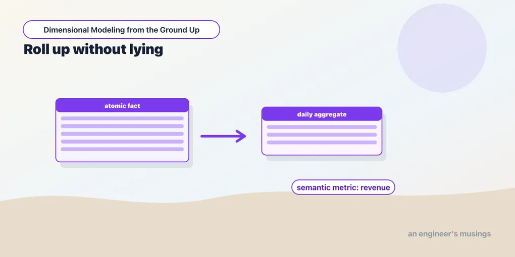
The first thing to get right is what an aggregate table is, because the wrong mental model — “a place to stash pre-baked numbers” — leads straight to tables that drift and can’t be checked. An aggregate fact table is a fact table. It has a declared grain, conformed dimensions, and additive measures, exactly like the atomic fact. The only difference is that its grain is deliberately coarser.

The bookshop’s atomic sales fact is one row per order line:

fct_order_items
grain: one row per order line
measures: quantity, extended_price

A day-grain aggregate collapses order lines into one row per book per day:

fct_book_sales_daily
grain: one row per book per day
measures: quantity, extended_price

The aggregate is not a replacement for the atomic table — you never throw the order lines away, because the day someone asks “which orders contained both a cookbook and a knife” you need line detail the rollup can’t reconstruct. The aggregate is a performance layer for the questions that genuinely don’t need line detail:

select
    date_sk,
    book_sk,
    sum(quantity) as quantity,
    sum(extended_price) as extended_price
from {{ ref('fct_order_items') }}
group by 1, 2

Two decisions are doing all the work here, and both come straight from the grain.

Which measures survive the rollup. Only additive ones. quantity and extended_price sum cleanly across any dimension, so they roll up for free. A ratio like margin percent does not — averaging an already-averaged margin gives you an average of averages, which is a different and wrong number. The rule from the fact-table chapter is the rule here: aggregate the additive components (margin dollars and cost dollars, separately) and let the ratio be recomputed from them, or don’t put the ratio in the aggregate at all and leave it to the semantic layer to compute at query time. An aggregate table full of pre-divided ratios is a trap.

When it’s worth building at all. Not every repeated query deserves an aggregate. Build one when a query is hot (run constantly — a landing dashboard, a daily executive email), coarse (asks for a rollup far above the atomic grain, so the aggregate is dramatically smaller than the source), and stable (the definition doesn’t churn weekly). A day-by-book rollup of a hundred-million-row order-line fact might be a few hundred thousand rows — a 100× to 1000× read reduction on every dashboard that touches it. A rollup that only shaves 2× off a query nobody runs twice is pure maintenance cost with no payoff. Aggregates are a cache, and caches earn their keep only where the hit rate is high.

Aggregate navigation, or the aggregate nobody has to know about

The uncomfortable part of aggregates is coupling. If a dashboard is hand-written against fct_book_sales_daily, then the day you ask for revenue by hour, the dashboard breaks — the aggregate doesn’t have the grain, and someone has to notice, rewrite the query against the atomic fact, and remember which questions are allowed to hit which table. Multiply that across dozens of dashboards and the aggregate becomes a liability: a second source of truth that consumers must route between by hand.

The classic solution is aggregate navigation (sometimes called query rewrite): a layer that accepts a query written against the atomic fact and silently redirects it to the smallest aggregate that can answer it. Ask for revenue by month and the navigator serves it from fct_book_sales_daily; ask for revenue by hour and it falls through to fct_order_items — same query, the router picks the table. The consumer never names the aggregate, so aggregates can be added, split, or dropped without touching a single dashboard. This is the feature that made 1990s ROLAP tools viable, and it’s the honest reason aggregates were ever manageable at scale: the coupling has to live in one place, not in every report.

This is also where the OLAP cube fits into the Kimball picture, because a cube is essentially an aggregate-navigation engine with the rollups precomputed for every combination of dimension levels at once. A cube over the sales star materializes sales by day-book, by month-category, by quarter-region, and so on up every hierarchy, then answers queries by reading the right cell. A star schema plus a handful of hand-chosen aggregate tables is the same idea done selectively — you precompute the rollups that are hot instead of all of them, trading cube completeness for a fraction of the storage and build cost. On a columnar cloud warehouse that scans fast and stores cheap, the selective approach usually wins, which is why explicit cube engines faded and aggregate tables (or their modern cousins, materialized views) stayed. The concept survived; the packaging changed.

Modern warehouses give you a piece of aggregate navigation for free. Snowflake’s materialized views and the automatic-clustering machinery, and the query optimizer’s ability to route a query to a materialized view that covers it, are aggregate navigation by another name — you define the rollup, and the optimizer decides when to use it. Worth checking against current Snowflake docs before leaning on it, because MV rewrite has real restrictions (limited aggregate functions, no outer joins in the MV definition), but where it applies it removes the routing problem entirely. Where it doesn’t, you build the aggregate as a dbt model and route to it deliberately — which brings us to building one that stays correct.

Rollups should be incremental

A day-grain aggregate over a growing fact should not fully rebuild every night — that throws away the whole point, which was to do the aggregation once. Build it incrementally, reprocessing only the recent slice that can still change:

{{ config(
    materialized='incremental',
    unique_key=['date_sk', 'book_sk']
) }}

with source_rows as (
    select *
    from {{ ref('fct_order_items') }}
    {% if is_incremental() %}
      where order_date >= current_date - 7
    {% endif %}
),

rolled as (
    select
        date_sk,
        book_sk,
        sum(quantity) as quantity,
        sum(extended_price) as extended_price
    from source_rows
    group by 1, 2
)

select * from rolled

The lookback window is the whole design, and getting it wrong is how an aggregate goes quietly wrong. Late-arriving facts change recent aggregates: an order corrected three weeks after the fact rewrites that day’s total, and if the incremental window only reaches back seven days, the correction never makes it into the rollup. The aggregate stays fast and becomes subtly stale — the most dangerous failure mode, because nothing errors. The rule is that an aggregate inherits the lateness behavior of its atomic fact. If orders can be corrected for thirty days, the aggregate’s lookback is thirty days, full stop. Match the window to the source’s actual volatility, not to what feels efficient.

For warehouses that partition, replacing every affected partition wholesale is often safer than a row-level merge, because it’s idempotent — rebuild the last thirty days of partitions from scratch and you can’t leave a half-updated row behind. The implementation is warehouse-specific (Snowflake leans on merge and delete+insert incremental strategies rather than explicit partitions); the design question is portable: what range of the aggregate can still change, and how do I rebuild exactly that range and nothing else?

Shrunken dimensions must be conformed, not private

Change the grain of the fact and you often change the grain of its dimensions too. A week-grain sales aggregate has no business joining to a day-grain dim_date — a week is seven calendar days, so a single aggregate row can’t point at one date_sk without either lying about which day it means or fanning out across seven. What it needs is a shrunken dimension: a dimension rolled up to match the coarser grain.

For a weekly rollup, that’s a week-grain calendar:

-- models/marts/dim_week.sql
select
    {{ dbt_utils.generate_surrogate_key(['iso_year', 'iso_week']) }} as week_sk,
    calendar_year,
    iso_week,
    calendar_quarter,
    min(date_day)  as week_start_date,
    max(date_day)  as week_end_date,
    count(*)       as days_in_week
from {{ ref('dim_date') }}
group by calendar_year, iso_week, calendar_quarter

And the weekly aggregate conforms to it:

-- models/marts/fct_book_sales_weekly.sql
{{ config(materialized='incremental', unique_key=['week_sk', 'book_sk']) }}

with lines as (
    select oi.*, d.calendar_year, d.iso_week
    from {{ ref('fct_order_items') }} oi
    join {{ ref('dim_date') }} d using (date_sk)
    {% if is_incremental() %}
      where oi.order_date >= current_date - 30
    {% endif %}
)

select
    {{ dbt_utils.generate_surrogate_key(['iso_year', 'iso_week']) }} as week_sk,
    book_sk,
    sum(quantity) as quantity,
    sum(extended_price) as extended_price
from lines
group by week_sk, book_sk

The load-bearing word is conformed. dim_week is not a private calendar the weekly aggregate invented for itself — it is built from dim_date, so its weeks, years, and quarters are the same weeks, years, and quarters every other star already uses. That matters because the whole reason to shrink a dimension rather than inline a couple of columns is so that a weekly sales aggregate and a weekly inventory aggregate can be sliced by the same dim_week and compared. The moment inventory rolls up to its own week table — one that starts weeks on Monday while sales starts on Sunday, say, because iso_week was computed two different ways — the two aggregates stop being comparable and the integration silently breaks. A shrunken dimension is a conformed dimension at a coarser grain; it is the same dimension, rolled up, derived from the atomic one so its meaning can’t drift. Building it from dim_date isn’t just convenient, it’s the mechanism that keeps conformance true. Kimball’s rule of thumb is worth stating plainly: a shrunken rollup dimension must be a strict subset of the base dimension’s rows and attribute values — never an independently sourced table that merely looks similar.

Shrinking also closes a specific bug. Join a week-grain fact to a day-grain dimension and, unless you’re careful, each aggregate row matches seven dimension rows and your revenue multiplies by seven. Matching the dimension’s grain to the fact’s grain makes that fan-out structurally impossible instead of something you have to remember not to do.

Drill-across is the query payoff

All of this conformance discipline exists to make one query pattern safe. When you want to compare two processes — units sold against units on hand, by title, by week — the wrong instinct is to join the two facts directly:

-- wrong: two facts at different grains, joined directly
from fct_order_items
join fct_inventory_daily using (book_sk, date_sk)

That fans out immediately, because fct_order_items is one row per order line and fct_inventory_daily is a periodic snapshot at one row per book per day — different grains, so the join multiplies. The correct pattern is drill-across: aggregate each fact to the common grain first, then join the two aggregates on their shared conformed keys:

with sales as (
    select date_sk, book_sk, sum(quantity) as units_sold
    from {{ ref('fct_order_items') }}
    group by 1, 2
),

inventory as (
    select date_sk, book_sk, max(stock_level) as units_on_hand
    from {{ ref('fct_inventory_daily') }}
    group by 1, 2
)

select
    d.date_day,
    b.title,
    sales.units_sold,
    inventory.units_on_hand
from sales
join inventory using (date_sk, book_sk)
join {{ ref('dim_date') }} as d using (date_sk)
join {{ ref('dim_book') }} as b using (book_sk)

Note the aggregations: sum(quantity) for sales because units sold add up across a day, but max(stock_level) for inventory because a stock level is a state, not a flow — you don’t sum today’s on-hand count across the week, you take the level at a point in time. That asymmetry is additivity showing up in the query, and it’s the same reason the semantic layer has to treat stock_level with care in a moment.

This query works only because both facts share a conformed dim_date and dim_book — the conformed-dimension chapter is the whole reason it’s coherent. Drill-across is what the bus matrix was for: two processes meeting on dimensions that agree.

The semantic layer over the star

An aggregate table can make extended_price fast. It should not be the only place the definition of “revenue” lives, and it definitely shouldn’t be the place three different dashboards each re-derive it. That’s the job of a semantic layer: name each metric once, above the tables, and make every consumer — BI tool, notebook, ad-hoc query — pull from that one definition. The star is the physical model; the semantic layer is the shared vocabulary on top of it.

dbt ships one: the dbt Semantic Layer, powered by MetricFlow. You describe your marts as semantic models (what entities, dimensions, and measures each fact exposes), then define metrics on top of those measures. MetricFlow compiles a request like “revenue by month” into the correct SQL — picking the joins, applying the aggregation, and, crucially, generating the same expression no matter who asks.

Start by describing the atomic sales fact:

# models/marts/semantic_models.yml
semantic_models:
  - name: order_items
    model: ref('fct_order_items')
    defaults:
      agg_time_dimension: order_date

    entities:
      - name: order_item
        type: primary
        expr: order_item_sk
      - name: order
        type: foreign
        expr: order_id
      - name: book
        type: foreign
        expr: book_sk
      - name: customer
        type: foreign
        expr: customer_sk

    dimensions:
      - name: order_date
        type: time
        type_params:
          time_granularity: day

    measures:
      - name: quantity
        description: "Units sold, at order-line grain."
        agg: sum
        expr: quantity
      - name: extended_price
        description: "Gross line amount."
        agg: sum
        expr: extended_price
      - name: order_count
        description: "Distinct orders."
        agg: count_distinct
        expr: order_id

Three things to notice. The entities are the surrogate keys the star already carries — order_item_sk is the primary entity, and book_sk/customer_sk are foreign entities that let MetricFlow join out to dim_book and dim_customer (defined as their own semantic models) to expose their attributes as queryable dimensions. The measures are the raw additive building blocks, each with its aggregation declared — this is where agg: sum says “this column is additive.” And agg_time_dimension: order_date tells MetricFlow which time column to roll up on by default, so “revenue by month” knows what “by month” means without you spelling it out every time.

Metrics then name the business-facing calculations on top of the measures:

# models/marts/metrics.yml
metrics:
  - name: revenue
    description: "Total gross sales amount."
    type: simple
    type_params:
      measure: extended_price

  - name: units_sold
    description: "Total units sold."
    type: simple
    type_params:
      measure: quantity

  - name: orders
    description: "Count of distinct orders."
    type: simple
    type_params:
      measure: order_count

  - name: average_order_value
    description: "Revenue per order."
    type: ratio
    type_params:
      numerator: revenue
      denominator: orders

revenue, units_sold, and orders are simple metrics — a name bolted onto a single measure. average_order_value is a ratio metric built from two other metrics, and this is the payoff. Average order value is a non-additive ratio: you can’t average it across segments, and you can’t precompute it in an aggregate table without pinning a grain. Defined as a ratio in the semantic layer, it’s computed correctly at query time for whatever grain the consumer asks — revenue-over-orders by month, by segment, by book category — each cut recomputed from its own numerator and denominator, never averaged from a pre-divided column. This is the class of metric a semantic layer handles that an aggregate table fundamentally can’t.

Additivity is the semantic layer’s problem too

The stock_level measure on fct_inventory_daily is the case that separates a semantic layer that understands dimensional modeling from one that just renames columns. stock_level is semi-additive: it adds up across books and stores (total units on hand across the catalog is a real number) but not across time (summing Monday’s, Tuesday’s, and Wednesday’s on-hand counts is meaningless — you’d triple-count the same physical books). It’s the classic balance-snapshot measure, and getting it wrong produces confidently wrong inventory numbers.

MetricFlow models this directly with a non_additive_dimension:

semantic_models:
  - name: inventory
    model: ref('fct_inventory_daily')
    defaults:
      agg_time_dimension: snapshot_date

    entities:
      - name: book
        type: foreign
        expr: book_sk

    dimensions:
      - name: snapshot_date
        type: time
        type_params:
          time_granularity: day

    measures:
      - name: stock_level
        description: "Units on hand — semi-additive over time."
        agg: sum
        non_additive_dimension:
          name: snapshot_date
          window_choice: max

agg: sum still governs the additive dimensions (sum across books and stores), while non_additive_dimension tells MetricFlow that across snapshot_date it must not sum — window_choice: max takes the level at the latest date in the queried window instead. Ask for inventory by month and you get the end-of-month stock level, not thirty days of levels added together. That’s the same max(stock_level) reasoning from the drill-across query, but now it’s declared once in the semantic model instead of being something every analyst has to remember to type. Encoding additivity in the layer is how you stop the semi-additive-measure bug at the source rather than catching it in review forever.

Querying it, and where it fits

With models and metrics defined, MetricFlow answers requests without anyone writing the join-and-group-by:

dbt sl query --metrics revenue,units_sold \
  --group-by metric_time__month,book__genre \
  --order-by metric_time__month

metric_time is MetricFlow’s cross-metric time dimension (the agg_time_dimension under the hood), so metric_time__month rolls both metrics to month; book__genre reaches through the book entity into dim_book for an attribute the sales fact never physically stored. The same query is available over the Semantic Layer’s APIs (JDBC, GraphQL) so a BI tool, a notebook, and a Slack bot all resolve “revenue by month” to identical SQL. That’s the consistency half of the chapter’s opening promise, delivered: one definition, many consumers, no drift.

Which raises the question the two techniques force: when does the semantic layer replace hand-built aggregate tables, and when doesn’t it?

It replaces them for definitional consistency and for non-additive metrics. Average order value, margin percent, any ratio or any metric whose correctness depends on grain — define these in the semantic layer and never materialize them, because a materialized ratio is a grain waiting to be queried wrong. The semantic layer computes them right at whatever grain is asked, which no single aggregate table can do.

It does not replace aggregates for raw latency on huge, hot rollups. A semantic-layer query for revenue by month still scans the atomic fact unless something underneath has precomputed the rollup — MetricFlow generates correct SQL, but correct SQL over a hundred-million-row fact is still a hundred-million-row scan. That’s exactly where you keep an aggregate table (or a materialized view), and the two compose: point the semantic model at a pre-aggregated mart, or let MetricFlow’s own caching and your warehouse’s MV rewrite serve the hot cuts, while the layer still guarantees the definition. Some Semantic Layer setups add declarative pre-aggregation so MetricFlow itself manages the rollups — check current dbt docs for what’s GA, since this surface moves fast. The durable split: the semantic layer owns what a metric means; aggregates and materialized views own how fast the common cut comes back. You want both, and they don’t compete.

Test aggregates against atomic facts

Every aggregate is a second copy of numbers that already exist atomically, and a second copy can disagree with the first. So reconcile them — sum the atomic fact to the aggregate’s grain and assert the totals match:

-- tests/assert_daily_aggregate_reconciles.sql
with atomic as (
    select date_sk, book_sk, sum(extended_price) as extended_price
    from {{ ref('fct_order_items') }}
    group by 1, 2
)

select
    atomic.date_sk,
    atomic.book_sk,
    atomic.extended_price as atomic_amount,
    agg.extended_price    as aggregate_amount
from atomic
full outer join {{ ref('fct_book_sales_daily') }} as agg
    using (date_sk, book_sk)
where coalesce(atomic.extended_price, 0) != coalesce(agg.extended_price, 0)

Zero rows means the aggregate agrees with the atomic source at the declared grain, in both directions — the full outer join catches a grain combination present in one table but missing from the other, which a plain inner join would silently skip. Without this test, an aggregate whose lookback window was too short drifts for weeks while dashboards stay fast and wrong, and nobody finds out until a total is questioned. Run it after the aggregate builds, on the same schedule, so the fast copy can never diverge from the true one for more than a night. The testing chapter makes the general case; this is its most important specific application, because an aggregate’s entire value proposition is being trusted without being checked.

One honesty note in keeping with the series: the MetricFlow YAML and dbt sl query shapes here are docs-correct for the current dbt Semantic Layer, and the SQL is standard Snowflake — but this series has no live Snowflake or Semantic Layer service to run against, so treat the semantic-layer snippets as verified-by-reading, and confirm the exact spelling of non_additive_dimension, metric_time, and the sl query flags against current dbt docs before you ship, since that surface is still moving.

Final thoughts

Aggregates and the semantic layer are not shortcuts around dimensional modeling — they’re dimensional modeling collecting its interest. The aggregate table is the star at a coarser grain, conforming to shrunken dimensions that were derived from the atomic ones so they can’t drift. The semantic layer is the star’s grain and additivity rules written down as executable definitions, so “revenue” and “average order value” and “units on hand” mean one thing across every tool that asks. Neither is possible without the discipline the rest of the series built: an aggregate needs a declared grain to reconcile against, a shrunken dimension needs a conformed base to derive from, and a semantic layer needs to know which measures are additive, semi-additive, or ratios before it can compute a single number correctly. Declare the grain, shrink dimensions when the grain changes, roll up only additive measures or their safe components, reconcile the fast copy against the true one every night, and define each metric exactly once above the tables. Speed is useful. Consistent speed is better. Correct, governed, consistent speed — the same number, fast, everywhere — is the point.

Next: Streaming Facts: When the Nightly Batch Stops Being Nightly