The Planner Is Guessing, and It Shows Its Work

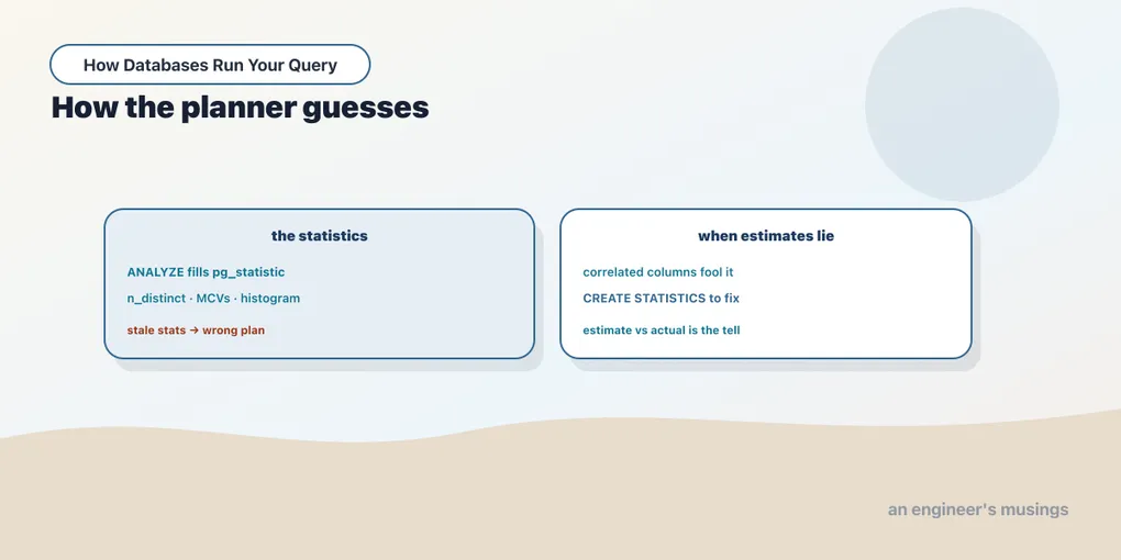
The planner picks a join algorithm from how many rows it thinks each side will produce, and it picks badly when those guesses are wrong. So where do the guesses come from? Not from running your query — that would defeat the purpose. They come from a small statistical summary of each table, one Postgres keeps current in the background and reads at planning time. This chapter opens that summary up, watches a stale one wreck a plan, and fixes a blind spot it has by design.

All of it was run against PostgreSQL 18. The estimate-versus-actual gaps below are real EXPLAIN ANALYZE output.

Where the numbers live

Run ANALYZE on a table and Postgres samples it, then stores a compact statistical profile in the system catalog pg_statistic. You read it through the friendlier view pg_stats. Three columns carry most of the weight.

n_distinct — how many distinct values a column has. Here’s the status column on orders:

SELECT attname, n_distinct, most_common_vals, most_common_freqs
FROM pg_stats WHERE tablename='orders' AND attname='status';

attname          | status
n_distinct       | 5
most_common_vals | {delivered,shipped,returned,placed,cancelled}
most_common_freqs| {0.41323334,0.1703,0.16776666,0.1652,0.0835}

Five distinct statuses, and the most-common-values list pairs each with its frequency: 41% of orders are delivered, 17% shipped, and so on. Now the planner can answer “how many rows match status = 'shipped'?” without touching the table — 17% of 60,000, about 10,200. That’s how a WHERE estimate gets made.

For a column with too many distinct values to list, Postgres keeps a histogram instead. Book prices:

SELECT attname, n_distinct, histogram_bounds
FROM pg_stats WHERE tablename='books' AND attname='price';

attname          | price
n_distinct       | -0.945
histogram_bounds  | {5.14,5.58,6.13,6.57,7.02,8.22,8.51,9.09,...}

Two things. The histogram bounds carve the values into buckets, each holding roughly the same number of rows. So the planner can estimate a range like price BETWEEN 20 AND 30 by counting buckets. And n_distinct is negative — that’s a ratio, not a count. -0.945 means “distinct values ≈ 94.5% of the row count,” i.e. prices are nearly unique. Postgres stores it as a ratio when distinctness scales with table size, so the estimate stays sane as the table grows.

Stale stats, bad plan

The statistics are only as good as the last ANALYZE. Autovacuum runs it periodically, but between a big data change and the next ANALYZE, the planner is working from an out-of-date picture. Let’s manufacture that gap. A scratch table of 100,000 rows, all one value:

CREATE TABLE events (id int, kind text, payload text);
INSERT INTO events SELECT g, 'common', 'x' FROM generate_series(1,100000) g;
CREATE INDEX events_kind_idx ON events(kind);
ANALYZE events;                        -- stats now say: kind is always 'common'

Now pour in 40,000 rows of a new value and, crucially, do not analyze:

INSERT INTO events SELECT g, 'rare', 'y' FROM generate_series(100001,140000) g;
EXPLAIN (ANALYZE, BUFFERS) SELECT count(*) FROM events WHERE kind='rare';

 Aggregate  (cost=4.32..4.33 rows=1) (actual time=9.443..9.444 rows=1.00 loops=1)
   ->  Index Only Scan using events_kind_idx on events
         (cost=0.29..4.31 rows=1) (actual time=0.023..7.643 rows=40000.00 loops=1)
         Index Cond: (kind = 'rare'::text)

Look at the estimate against the reality: rows=1 planned, rows=40000 actual. The planner has never heard of 'rare' — its stats still say the column is 100% 'common' — so it assumed the value barely exists and estimated a single row. A forty-thousand-fold miss. On this query the damage is mild. But an estimate this wrong is exactly what makes the join planner reach for a nested loop over 40,000 rows, or skip an index it should have used.

Now run ANALYZE and ask again:

ANALYZE events;
SELECT n_distinct, most_common_vals, most_common_freqs
  FROM pg_stats WHERE tablename='events' AND attname='kind';

 n_distinct | most_common_vals | most_common_freqs
------------+------------------+-------------------------
          2 | {common,rare}    | {0.71243334,0.28756666}

 Index Only Scan ... (cost=0.29..1065.83 rows=40259) (actual rows=40000.00 loops=1)

The estimate is now 40,259 against 40,000 actual — dead on. ANALYZE re-sampled, found 'rare' making up 29% of the table, and the guess snapped into place. Nothing about the data changed; only the planner’s knowledge of it did.

When a bad estimate flips the whole plan

The count query above kept the same plan shape. Here’s one where the stale estimate changes the strategy. A skewed table joined to a tiny lookup:

CREATE TABLE kind_dim (kind text PRIMARY KEY, label text);
INSERT INTO kind_dim VALUES ('a','Alpha'),('b','Beta');
CREATE TABLE skew (id int, kind text);
INSERT INTO skew SELECT g, 'a' FROM generate_series(1,1000) g;
ANALYZE skew;                          -- stats say: 1000 rows, all 'a'
INSERT INTO skew SELECT g,'b' FROM generate_series(1001,81000) g;  -- 80k 'b', not analyzed

With stale stats, the planner thinks kind='b' matches essentially nothing:

 Nested Loop  (cost=0.00..1257.54 rows=1) (actual time=0.070..83.344 rows=80000.00 loops=1)
   ->  Seq Scan on skew s (rows=1 planned) (actual rows=80000.00 loops=1)
         Filter: (kind = 'b'::text)
   ->  Seq Scan on kind_dim d (actual rows=1.00 loops=80000)
 Execution Time: 86.683 ms

It put skew on the outside of a nested loop, expecting one row, and drove 80,000 loops through the inner scan. 86 milliseconds, and it read 80,359 buffer pages doing it. Now ANALYZE skew and rerun:

 Nested Loop  (cost=0.00..2172.53 rows=80001) (actual time=0.069..11.501 rows=80000.00 loops=1)
   ->  Seq Scan on kind_dim d (actual rows=1.00 loops=1)
   ->  Seq Scan on skew s (rows=80001 planned) (actual rows=80000.00 loops=1)
 Execution Time: 15.055 ms

Same join, reshaped completely. Now that it knows skew returns 80,000 rows, the planner flips the sides. It scans the tiny kind_dim once as the outer, and reads skew a single time as the inner. loops collapsed from 80,000 to 1, buffer reads from 80,359 to 360, and the time from 86ms to 15ms. The only thing that changed was a fresh ANALYZE.

The blind spot: correlated columns

There’s one class of misestimate that a fresh ANALYZE won’t fix, because the statistics we’ve seen are per-column. Postgres keeps a profile for each column independently, and to estimate A AND B it multiplies their individual selectivities — which is correct only if A and B are independent. Often they aren’t. Consider a table where city fully determines region:

CREATE TABLE shipments AS
SELECT g AS id, 'city_'||(g%100) AS city, 'region_'||(g%100) AS region
FROM generate_series(1,100000) g;
ANALYZE shipments;
EXPLAIN ANALYZE
SELECT * FROM shipments WHERE city='city_7' AND region='region_7';

 Seq Scan on shipments  (cost=0.00..2140.00 rows=10) (actual rows=1000.00 loops=1)
   Filter: ((city = 'city_7') AND (region = 'region_7'))

rows=10 estimated, 1000 actual — a hundred-fold miss, on freshly analyzed data. The planner reasoned: city_7 is 1 in 100, region_7 is 1 in 100, so together 1 in 10,000, times 100,000 rows equals 10. But city_7 always comes with region_7 — the second condition filters out nothing. The columns are perfectly correlated, and multiplying their selectivities double-counts the filter.

The fix is extended statistics: tell Postgres to track the two columns together.

CREATE STATISTICS shipments_city_region (dependencies, ndistinct) ON city, region FROM shipments;
ANALYZE shipments;
EXPLAIN ANALYZE
SELECT * FROM shipments WHERE city='city_7' AND region='region_7';

 Seq Scan on shipments  (cost=0.00..2140.00 rows=997) (actual rows=1000.00 loops=1)

rows=997 against 1000 actual. The estimate went from 10 to 997 the moment Postgres knew the columns were linked. You can see the dependency it learned:

SELECT stxname, stxddependencies FROM pg_statistic_ext s
  JOIN pg_statistic_ext_data d ON d.stxoid = s.oid
  WHERE stxname='shipments_city_region';

 shipments_city_region | {"2 => 3": 1.000000, "3 => 2": 1.000000}

"2 => 3": 1.000000 reads as “column 2 (city) fully determines column 3 (region)” — dependency degree 1.0. With that recorded, the planner stops multiplying and estimates correctly. Reach for CREATE STATISTICS whenever two columns in a WHERE are related — city/region, country/currency, make/model — and the plans start blaming a bad estimate.

Final thoughts

The planner is a guessing machine, and pg_stats is what it guesses from. Two failure modes cover most bad plans: the statistics are stale, so re-run ANALYZE; or the statistics are per-column and your predicate spans correlated columns, so add extended statistics. A slow query with a wildly wrong row estimate in its plan is almost never a query problem. It’s a statistics problem wearing a query’s clothes. Next we go one layer down, to how a row even exists while other transactions are reading and writing it.

Next: Readers never block writers: MVCC — the trick that lets a long read and a live write touch the same row at the same time.