Beyond the B-tree: GIN, GiST, and BRIN

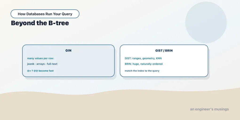
A B-tree indexes a value: one row, one key, sorted. That covers most columns, but not all of them. Some columns hold values with many keys inside — a JSONB document with a dozen fields, an array of tags, a paragraph of searchable text. You cannot sort a document into a B-tree in a way that answers “which rows contain the tag signed,” because that question is about the document’s contents, not its order. Postgres has index types built exactly for this. GIN indexes the many keys inside a value. GiST indexes things with extent, like ranges and shapes. And BRIN indexes enormous naturally-ordered tables for a rounding error of space. This chapter shows each turning a full scan into an index scan, against real data.

GIN: many keys per row

GIN stands for Generalized Inverted Index, and “inverted” is the important word. A B-tree maps a row to its value. An inverted index does the reverse: it maps each key back to the rows that contain it, the way a book index maps each term to its pages. That is precisely what you want for a document column.

Build a scratch table of 80,000 book events, each with a JSONB payload of genre, tags, and rating. Seed a rare tag misprint on a couple hundred rows — the realistic case of hunting for a scarce attribute:

SELECT count(*) FROM book_events WHERE payload @> '{"tags":["misprint"]}';
-- 200

The @> operator asks “does the left JSONB contain the right one.” Without an index, answering it means deserializing and checking all 80,000 documents:

EXPLAIN (ANALYZE, BUFFERS)
SELECT event_id, book_id FROM book_events WHERE payload @> '{"tags":["misprint"]}';

 Seq Scan on book_events  (cost=0.00..4221.00 rows=208 width=12)
                          (actual time=0.012..32.307 rows=200.00 loops=1)
   Filter: (payload @> '{"tags": ["misprint"]}'::jsonb)
   Rows Removed by Filter: 79800
   Buffers: shared hit=3221
 Execution Time: 32.349 ms

32 ms, 3,221 pages, to return 200 rows. Now index the column with GIN:

CREATE INDEX idx_be_payload ON book_events USING gin (payload);
ANALYZE book_events;

EXPLAIN (ANALYZE, BUFFERS)
SELECT event_id, book_id FROM book_events WHERE payload @> '{"tags":["misprint"]}';

 Bitmap Heap Scan on book_events  (cost=51.17..724.41 rows=213 width=12)
                                 (actual time=0.119..0.189 rows=200.00 loops=1)
   Recheck Cond: (payload @> '{"tags": ["misprint"]}'::jsonb)
   Heap Blocks: exact=6
   Buffers: shared hit=13
   ->  Bitmap Index Scan on idx_be_payload  (cost=0.00..51.12 rows=213 width=0)
                                            (actual time=0.104..0.104 rows=200.00 loops=1)
         Index Cond: (payload @> '{"tags": ["misprint"]}'::jsonb)
 Execution Time: 0.236 ms

From 32.3 ms to 0.236 ms, and from 3,221 pages to 13. The GIN index stored an entry for every distinct key and value across all 80,000 documents, so it can jump straight to the 200 rows carrying misprint. Note the node is a Bitmap Index Scan, always. GIN never produces a plain index scan the way a B-tree does. It returns a set of matching row locations with no useful ordering, and those always feed a bitmap heap scan. Seeing a bitmap here is correct, not a fallback.

GIN for full text

The same index type powers full-text search. Text search matches a tsvector (a document reduced to normalized lexemes) against a tsquery using the @@ operator. Over the event descriptions, searching for “railways” without an index means computing to_tsvector on every row:

EXPLAIN (ANALYZE)
SELECT count(*) FROM book_events WHERE to_tsvector('english', descr) @@ to_tsquery('english', 'railways');

 Finalize Aggregate  (actual time=269.553..271.849 rows=1.00 loops=1)
   ->  Gather (Workers Launched: 2)
         ->  Parallel Seq Scan on book_events  (actual time=1.247..262.431 rows=5333.33 loops=3)
               Filter: (to_tsvector('english'::regconfig, descr) @@ '''railway'''::tsquery)
 Execution Time: 271.899 ms

272 ms, and Postgres even threw two parallel workers at it. An expression GIN index — one built on the to_tsvector expression itself — precomputes the vector once per row and indexes its lexemes:

CREATE INDEX idx_be_fts ON book_events USING gin (to_tsvector('english', descr));
ANALYZE book_events;

 Finalize Aggregate  (actual time=12.764..13.221 rows=1.00 loops=1)
   ->  Parallel Bitmap Heap Scan on book_events  (actual time=1.697..4.745 rows=5333.33 loops=3)
         Recheck Cond: (to_tsvector('english'::regconfig, descr) @@ '''railway'''::tsquery)
         ->  Bitmap Index Scan on idx_be_fts (actual time=4.716..4.717 rows=16000.00 loops=1)
 Execution Time: 13.271 ms

272 ms down to 13 ms. The lexemes are precomputed and indexed, so the query looks up railway instead of tokenizing 80,000 strings. (The query term railways stems to railway, which is why the index condition shows the stem.) One rule to internalize: the index expression must match the query’s expression exactly. Index to_tsvector('english', descr) and query with the same call, or the index will not be used.

GiST: ranges, geometry, nearest-neighbour

GiST — Generalized Search Tree — is a framework for indexing data that has extent rather than a single sortable value: ranges, geometric shapes, IP networks, and full-text with ranking. Its natural home is the overlap and containment questions a B-tree can’t express.

Build 50,000 promotions, each a daterange of when it ran, and ask which were active on a given day. The @> operator here means “does this range contain this date.” Without an index it is a full scan:

EXPLAIN (ANALYZE) SELECT count(*) FROM promotions WHERE during @> DATE '2025-06-15';

 Aggregate  (actual time=6.349..6.349 rows=1.00 loops=1)
   ->  Seq Scan on promotions  (actual time=0.033..6.261 rows=1946.00 loops=1)
         Filter: (during @> '2025-06-15'::date)
         Rows Removed by Filter: 48054

A GiST index on the range column changes that:

CREATE INDEX idx_promo_during ON promotions USING gist (during);
ANALYZE promotions;

 Aggregate  (actual time=0.833..0.833 rows=1.00 loops=1)
   ->  Bitmap Heap Scan on promotions  (actual time=0.304..0.756 rows=1946.00 loops=1)
         Recheck Cond: (during @> '2025-06-15'::date)
         ->  Bitmap Index Scan on idx_promo_during  (actual time=0.278..0.278 rows=1946.00 loops=1)
               Index Cond: (during @> '2025-06-15'::date)
 Execution Time: 0.888 ms

6.4 ms to 0.888 ms. Each GiST tree node stores a bounding box covering its children, so a search descends only into subtrees whose box could contain the target date, skipping the rest. That bounding-box idea generalizes. The same structure answers “which shapes overlap this rectangle” for the PostGIS spatial types. And it uniquely supports nearest-neighbour search: ORDER BY location <-> point LIMIT 10 returns the ten closest rows using the index, which no B-tree can do. GiST also backs exclusion constraints, the clean way to say “no two promotions for the same genre may overlap in time.” A related type, SP-GiST, handles data that partitions naturally (quadtrees, IP prefixes); reach for it when the docs point you there.

One extension note. Indexing a scalar column and a range together — say (genre, during) in one GiST index — needs the btree_gist extension (CREATE EXTENSION btree_gist). It teaches GiST to handle ordinary types alongside ranges, and ships with Postgres but is not installed by default.

BRIN: enormous and ordered, for almost nothing

The last type is the specialist. BRIN — Block Range Index — does not store row locations at all. It stores, for each block range of the table, the min and max of the indexed column. If your query wants order_id BETWEEN 1000 AND 2000 and BRIN knows block range 5 holds ids 40,000–41,000, it skips that range entirely. This only works when the column’s values track physical storage order — a timestamp on an append-only log, an auto-incrementing id — but when they do, the size is astonishing. On the naturally-ordered order_items:

   relname    | pg_size_pretty
--------------+----------------
 idx_oi_brin  | 24 kB
 idx_oi_btree | 2392 kB

The BRIN index is 24 kB against the B-tree’s 2.4 MB, a hundredfold smaller. It stores a summary per block range instead of an entry per row. BRIN trades precision for size: it narrows the scan to candidate block ranges, then rechecks each row. On a billion-row time-series table where a B-tree would be gigabytes, a BRIN is megabytes and still prunes most of the table. The catch is the ordering requirement; on a randomly-ordered column, BRIN’s ranges all overlap and it prunes nothing.

A portability note to close the index tour. GIN, GiST, SP-GiST, and BRIN are largely Postgres-specific names. Other engines reach the same goals by other routes: MySQL has FULLTEXT indexes and spatial R-tree indexes; SQLite has FTS5 as a separate module. The concepts — inverted indexing for many-keyed values, tree-of-bounding-boxes for extents, block summaries for ordered bulk — travel further than the syntax.

Final thoughts

When a B-tree can’t help, the shape of the data tells you which index can. Many keys inside one value — JSONB, arrays, full text — want GIN, which always drives a bitmap scan. Ranges, geometry, and nearest-neighbour want GiST and its bounding boxes. Huge naturally-ordered tables want BRIN, which indexes for almost nothing by summarizing block ranges. We have now covered how the database finds rows. The other half of a query’s cost is combining rows from different tables, and that comes down to which of three join algorithms the planner picks.

Next: Three ways to join