The B-tree That Finds a Row
The B-tree index, shown before and after: a selective lookup as a full-table scan, then the same query as an index scan once the index exists, with the real timing drop. When an index earns its keep, when the planner ignores it, and what it costs you. Run against PostgreSQL 18.
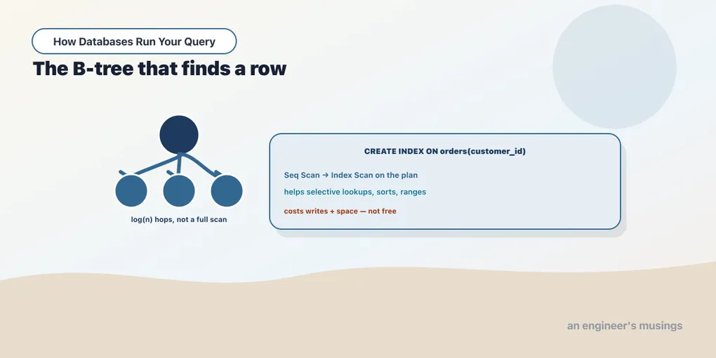
An index is the single biggest lever you have over query speed, and it is worth understanding what one actually is before reaching for it. The default index in every relational database is a B-tree: a balanced tree, sorted by the indexed column. It lets the database find a value in a handful of steps instead of scanning the whole table. Think of the index at the back of a book. To find every mention of “mitochondria” you do not read all 400 pages; you flip to M, read off the page numbers, and turn straight to them. A B-tree is that index, kept sorted and shallow so any lookup takes only a few hops from root to leaf.
The best way to feel what an index does is to measure the same query with and without one. We start from a table with no index where it matters, watch a query crawl, add the index, and watch it fly.
Before: the selective scan
The orders table has a primary-key index on order_id and nothing else. Asking for one customer’s orders means filtering on customer_id, which is unindexed:
EXPLAIN (ANALYZE, BUFFERS) SELECT * FROM orders WHERE customer_id = 42; QUERY PLAN
--------------------------------------------------------------------------------
Seq Scan on orders (cost=0.00..1133.00 rows=12 width=21)
(actual time=0.710..3.026 rows=8.00 loops=1)
Filter: (customer_id = 42)
Rows Removed by Filter: 59992
Buffers: shared hit=383
Execution Time: 3.062 msCustomer 42 placed 8 orders. To find them, Postgres read all 60,000 rows and threw away 59,992 (Rows Removed by Filter). It touched all 383 pages of the table to return eight rows. This is the query that gives sequential scans their bad name: a tiny, selective result — a small fraction of the table — fetched by reading everything. The work is wildly out of proportion to the answer, and that disproportion is exactly what an index removes.
After: create the index
One statement builds the B-tree, and one ANALYZE refreshes the statistics so the planner costs it with current information:
CREATE INDEX idx_orders_customer ON orders(customer_id);
ANALYZE orders;
Now run the identical query:
EXPLAIN (ANALYZE, BUFFERS) SELECT * FROM orders WHERE customer_id = 42; QUERY PLAN
------------------------------------------------------------------------------------
Bitmap Heap Scan on orders (cost=4.38..46.16 rows=12 width=21)
(actual time=0.032..0.054 rows=8.00 loops=1)
Recheck Cond: (customer_id = 42)
Heap Blocks: exact=8
Buffers: shared hit=8 read=2
-> Bitmap Index Scan on idx_orders_customer (cost=0.00..4.38 rows=12 width=0)
(actual time=0.019..0.020 rows=8.00 loops=1)
Index Cond: (customer_id = 42)
Buffers: shared hit=8 read=2
Execution Time: 0.096 msFrom 3.062 ms to 0.096 ms, about thirtyfold, and the buffer count fell from 383 to 10. The query now touches ten pages instead of every page in the table. That is the index earning its keep.
The plan is not quite the plain “Index Scan” you might expect, and the reason is worth a moment. Postgres chose a Bitmap Heap Scan fed by a Bitmap Index Scan. The bottom node walks the B-tree, collects the locations of all eight matching rows, and builds a bitmap of the pages that hold them. The top node then reads those pages in physical order. Postgres picks this variant when the matching rows are scattered across several pages, as they are here: eight rows in eight different Heap Blocks. Reading those pages in disk order is cheaper than bouncing back and forth. The Recheck Cond is bookkeeping for that bitmap. It is still an index-driven plan; it just adds a sorting-of-pages step on top.
To see a plain Index Scan, ask for something the index can satisfy in its own sorted order:
EXPLAIN (ANALYZE, BUFFERS) SELECT * FROM orders ORDER BY customer_id LIMIT 5; QUERY PLAN
------------------------------------------------------------------------------------------
Limit (cost=0.29..0.51 rows=5 width=21) (actual time=0.067..0.085 rows=5.00 loops=1)
-> Index Scan using idx_orders_customer on orders
(cost=0.29..2700.28 rows=60000 width=21) (actual time=0.066..0.083 rows=5.00 loops=1)
Execution Time: 0.161 msHere the index is walked in order and the LIMIT stops it after five rows. No sort, no filter, no scanning 60,000 rows to find the smallest five. This is the second thing an index buys you, and it is easy to miss. Because a B-tree is sorted, it can satisfy an ORDER BY on the indexed column for free. It can also answer a range query like customer_id BETWEEN 40 AND 50 by walking a contiguous stretch of leaves. An index is not only for equality lookups. Selective equality, ranges, and sorts are all its home turf.
When the planner ignores the index
An index is an option, not an obligation. The planner uses it only when its cost model says the index is cheaper, and for a query that wants most of the table, it is not. Ask for every order from the first 4,000 customers:
EXPLAIN (ANALYZE, BUFFERS) SELECT * FROM orders WHERE customer_id < 4000; QUERY PLAN
-----------------------------------------------------------------------------------
Seq Scan on orders (cost=0.00..1133.00 rows=48076 width=21)
(actual time=0.008..4.515 rows=48014.00 loops=1)
Filter: (customer_id < 4000)
Rows Removed by Filter: 11986
Execution Time: 6.051 msThe index still exists. The planner ignored it and chose a sequential scan, because this filter keeps 48,014 of 60,000 rows — 80% of the table. Using the index would mean walking almost the entire B-tree and then fetching almost every page anyway, which is more work than reading the table straight through. The planner priced both and the scan won. This is the mirror image of the first query: same table, same index, but a non-selective predicate flips the right answer back to a full scan.
The principle underneath both cases is selectivity. An index pays off when the query wants a small fraction of the rows, and stops paying somewhere in the low tens of percent. The exact crossover depends on how the rows are physically clustered, which is why you let the planner decide from statistics rather than forcing an index by hand. When a query that should be selective still scans, the usual culprit is stale statistics or a predicate the index can’t serve. That is the kind of estimate gap the previous chapter showed.
What the index costs
An index is not free, and the price is easy to forget because it is paid elsewhere. First, space:
SELECT pg_size_pretty(pg_relation_size('idx_orders_customer')) AS idx_size,
       pg_size_pretty(pg_relation_size('orders'))              AS table_size;
idx_size | table_size
----------+------------
536 kB | 3064 kBThe index is a real, separate structure on disk, about a sixth of the table here and larger on wider keys. Second, and more important, write cost. Every INSERT into orders, and every UPDATE that changes customer_id, must now also update this B-tree to keep it sorted and balanced. An index speeds reads by slowing writes. On a table that is written far more than it is read, or indexed on a column nobody filters by, that trade goes the wrong way. The discipline is to index the columns your queries actually filter, join, and sort on, and no others. An unused index is pure overhead: it costs space and slows every write while helping no query.
The syntax is standard across engines. MySQL and SQL Server both spell it CREATE INDEX, and both default to a B-tree, though the plan output and the exact clustering rules differ. The mental model transfers cleanly: a sorted side structure that trades write speed and space for fast selective reads.
Final thoughts
A B-tree index turns a selective lookup from a full-table scan into a direct jump. We watched customer_id = 42 drop from 3 ms and 383 pages to a tenth of a millisecond and 10 pages the moment the index existed. And we watched the planner correctly decline the index when a query wanted 80% of the table. Index the columns you filter, range, join, and sort on; pay for it in write speed and space; and let the planner choose when to use it. A single-column B-tree is the foundation. Next we make indexes do more with less: covering several columns at once, carrying extra columns to skip the table entirely, and indexing only the rows you care about.
Next: Indexes that do more
Comments