Appendix A: Where These Models Came From

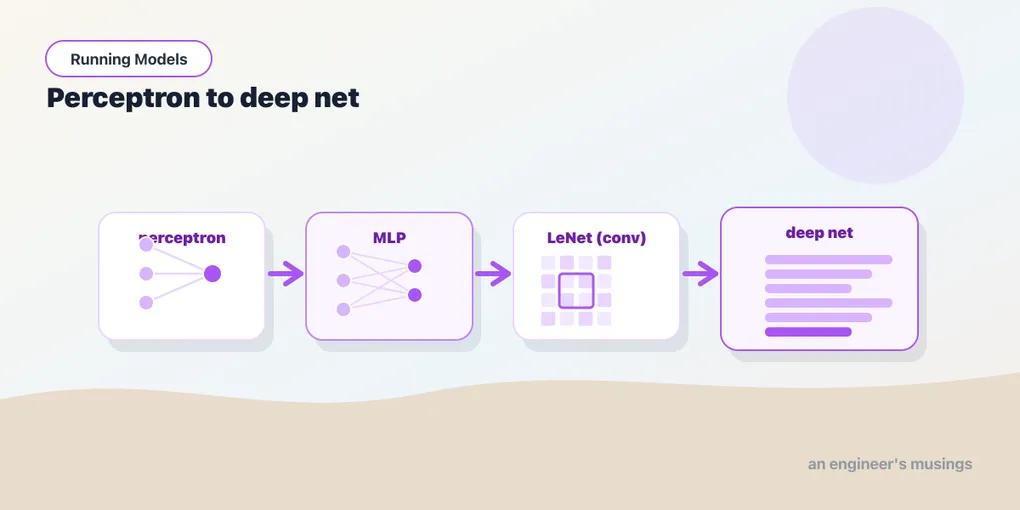
Nothing in this appendix is needed to run a model, which is why it is an appendix. It is here because the shapes you read in Part II — a single Linear, a small stack, a sandwich of convolutions, a block of attention — are not arbitrary. Each one is a famous model, and the trail from the first to the last is short and worth knowing. Every model below is a handful of lines you can build and print; none of them is trained, and that is the point.

▶ Open the companion notebook in Colab

Run against: PyTorch 2.2.2 on CPU (macOS).

The perceptron: a single layer, in 1958

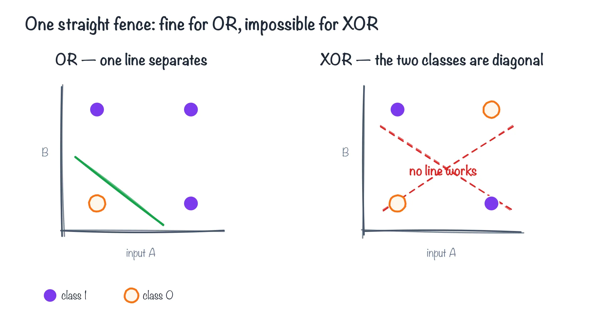
One straight line can fence off OR’s lone corner, but no single line separates XOR’s diagonal classes.

In 1958 Frank Rosenblatt unveiled the perceptron, and within a couple of years had built it into a genuine machine — the Mark I Perceptron, a room of wires and motor-driven dials that learned to tell simple shapes apart through a camera. Strip away the hardware and the idea is one you know cold from chapter 11: take some inputs, multiply each by a weight, add them up, and fire a 1 if the total clears a threshold, else a 0. A weighted sum, then a yes/no.

That’s a single nn.Linear with a threshold stuck on the end:

import torch
import torch.nn as nn

perceptron = nn.Linear(2, 1)        # two inputs, one output — Rosenblatt's unit
score = perceptron(torch.tensor([[1.0, 1.0]]))
print(score)                        # a weighted sum; the perceptron fires 1 if it's > 0

If that weighted sum looks familiar, it should: with a single input it’s just y = mx + b — the equation of a line, with the weight as the slope m and the bias as the intercept b. The twist is what the perceptron does with it. It doesn’t read off a y value (that’s what linear regression, in the next section, will do) — it checks which side of the line you land on: w·x + b > 0 fires a 1, everything else a 0. The same line equation, used as a fence between two classes rather than a prediction. That’s also the seed of its famous limitation — a single straight fence can only separate so much.

The perceptron caused a sensation — newspapers wrote about a machine that might one day “walk, talk, see, write.” Then in 1969 Marvin Minsky and Seymour Papert published a book, Perceptrons, with a quietly devastating observation: a single layer like this cannot learn XOR — the simple rule “one or the other, but not both.” No setting of two weights and a threshold can draw the line, because no straight line separates the cases. The result helped cool the early hype: funding and attention drifted away from perceptron-style networks, and the lean years that followed are often called a neural-network “winter.” (Historians still argue over how much the book itself was to blame — plenty else was going on — but the chill was real.)

Hold on to that limitation, because the fix is sitting in chapter 11.

Linear and logistic regression: one layer, doing real work

Before we fix it, notice that the single layer was never useless — drop the hard threshold and it’s a workhorse you’ve definitely met.

A bare nn.Linear, no activation, is linear regression — the line-of-best-fit from every statistics class:

linreg = nn.Linear(4, 1)            # 4 features in, one number out

Put a sigmoid on the end — a smooth squash into the range 0 to 1 — and you have logistic regression, the most widely used classifier on the planet, the thing predicting spam-or-not and click-or-not in a million production systems:

logreg = nn.Sequential(
    nn.Linear(4, 1),                # weighted sum
    nn.Sigmoid(),                   # squash to a probability between 0 and 1
)
print(logreg(torch.rand(1, 4)))     # e.g. tensor([[0.62]]) — a probability

Swap the sigmoid for a softmax over several outputs and you get softmax regression — which is exactly the single-Linear-plus-softmax classifier that caps nearly every model in this book, from ResNet’s fc to DistilBERT’s classifier. The lesson: one layer, depending on what you tack onto the end, is regression, a probability, or a classifier. It’s a small tool that does a startling amount of real work.

The hidden layer that changed everything

Now the fix. Minsky and Papert were right that one layer can’t do XOR — but stack a second layer between input and output, with a nonlinear ReLU in the middle, and the wall comes down. That extra layer is called a hidden layer, and a network with one is a multi-layer perceptron (MLP). You built one in chapter 11:

xor_net = nn.Sequential(
    nn.Linear(2, 2),                # a hidden layer of 2 units
    nn.ReLU(),                      # the nonlinear kink that makes depth count
    nn.Linear(2, 1),
)
print(xor_net)

Once trained (training is the Training Models book — here we just build the shape), this two-layer net solves the very problem that sank the perceptron. And it’s not a one-trick fix. The Universal Approximation Theorem (Cybenko, 1989; Hornik, 1991) proved something remarkable about exactly this shape: a single hidden layer, given enough units, can approximate any continuous function to whatever accuracy you like. One hidden layer is, in principle, enough to represent almost anything.

So why go deeper than one hidden layer? Because “in principle” can demand an absurdly wide layer, while stacking layers builds complexity efficiently — each layer composing on the last. That insight, plus a way to actually train the stacks (backpropagation, popularized in 1986), is the whole ballgame. “Deep learning” is just this: more hidden layers.

LeNet: the first sandwich, in twelve lines

Every layer so far treats its input as a flat, unordered list, which chapter 12 showed is a quiet disaster for images. The fix there was convolution, and the first network to use it for a real job was LeNet-5 (Yann LeCun, 1998), which read handwritten digits well enough to sort mail and cash cheques. It’s the same nn.Sequential you know, with the vision layers in the mix:

lenet = nn.Sequential(
    nn.Conv2d(1, 6, kernel_size=5, padding=2),  # slide 6 filters over a 1-channel image
    nn.ReLU(),
    nn.MaxPool2d(2),                            # halve the height and width
    nn.Conv2d(6, 16, kernel_size=5),
    nn.ReLU(),
    nn.MaxPool2d(2),
    nn.Flatten(),                               # grid -> a flat row, to hand to Linear
    nn.Linear(16 * 5 * 5, 120),
    nn.ReLU(),
    nn.Linear(120, 84),
    nn.ReLU(),
    nn.Linear(84, 10),                          # 10 outputs — one per digit, 0 through 9
)

total = sum(p.numel() for p in lenet.parameters())
print(f"{total:,} parameters")                  # 61,706 parameters
print(lenet(torch.rand(1, 1, 28, 28)).shape)    # torch.Size([1, 10])

Read it top to bottom and it’s exactly chapter 12’s sandwich: two Conv2d+ReLU+MaxPool2d stages that see, a Flatten, then three Linear layers that decide, ending in 10 outputs — one per digit. And look at the count: 61,706 parameters for the whole thing, against the 785,000 a single flat Linear layer wanted for the same image. Convolution didn’t just see better; it did it with a fraction of the weights. ResNet-18 is this idea stacked far deeper, with a trick (the “residual” connection) that lets the stack go deep without the signal fading.

A transformer block, built and counted

Chapter 13 described the transformer block on paper; here it is as code. PyTorch ships one ready-made, nn.TransformerEncoderLayer, and sized to the twelve-word toy it is tiny:

embed = nn.Embedding(12, 4)                  # the chapter 13 lookup: a 12-word vocab, 4 numbers per word
ids = torch.tensor([[0, 2, 4, 6, 0, 7]])     # "the cat sat on the mat", batched
emb = embed(ids)                             # [1, 6, 4] — six word-vectors

block = nn.TransformerEncoderLayer(
    d_model=4,              # match the embedding width
    nhead=2,                # heads split d_model into equal parts, so it must divide 4
    dim_feedforward=8,      # the little MLP's hidden size
    batch_first=True,
)
print(block(emb).shape)                                   # torch.Size([1, 6, 4])
print(sum(p.numel() for p in block.parameters()))         # 172

Same shape in, same shape out, 172 numbers. Now scale it to the width a real model uses and print it:

block = nn.TransformerEncoderLayer(d_model=128, nhead=8, dim_feedforward=512, batch_first=True)
print(block)
print(f"{sum(p.numel() for p in block.parameters()):,} parameters")   # 198,272 parameters

TransformerEncoderLayer(
  (self_attn): MultiheadAttention(
    (out_proj): NonDynamicallyQuantizableLinear(in_features=128, out_features=128, bias=True)
  )
  (linear1): Linear(in_features=128, out_features=512, bias=True)
  (dropout): Dropout(p=0.1, inplace=False)
  (linear2): Linear(in_features=512, out_features=128, bias=True)
  (norm1): LayerNorm((128,), eps=1e-05, elementwise_affine=True)
  ...
)

There it is: self_attn (the new idea), two Linear layers (the feed-forward network), and the LayerNorms (the supporting cast). Widen d_model from 4 to 128 and the count climbs from 172 to about two hundred thousand, all of it random and untrained here. DistilBERT, which you read in chapter 14, is six of these at width 768 behind an embedding table; GPT-2 is twelve, facing the other way. The whole zoo is this block, stacked.

The thread

Stand back and the lineage is one idea, growing up:

• Perceptron — one weighted sum and a threshold. Couldn’t do XOR.
• Logistic regression — the same one layer with a smooth squash; a probability machine still everywhere in production.
• MLP — add a hidden layer and a nonlinearity; now it can approximate anything, XOR included.
• LeNet — give the layers a window onto the image, and they can see.
• The transformer block — give every position a view of every other, and they can read.

Every step is the previous one plus one idea, and every step is built from pieces you assembled by hand in Part II. The famous models aren’t a different species; they’re the toy, scaled.

Back to the Running Models series.