The Economics of Small Models

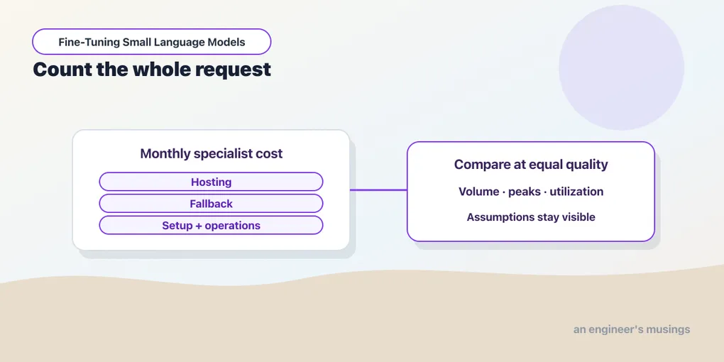
A model that costs less per token can still make the system more expensive — it may require an always-on server, a second call for difficult requests, a labeling process, and someone to investigate regressions. At low volume, those fixed costs can dominate the entire bill.

The bookshop has three possible arrangements: send each request to an API, host a larger general model, or operate small specialists with a fallback path. Each comparison needs the same unit of work: an answered customer request, including any extraction, SQL execution, and review after routing.

The question is what an acceptable completed request costs under our workload and service target. Model size contributes — alongside traffic shape, answer quality, and the work of keeping enough capacity available to serve requests dependably.

Run against: Python 3.13.3; companion operations.py cost calculator, replica-boundary checks, and cost-scenarios.json.

Not run. Provider billing, production throughput, concurrency, energy consumption, and staffed operating costs were not measured.

Every dollar rate and serving-capacity input in the scenario below is an explicit hypothetical assumption. The table is an arithmetic comparison, not a current price quote or purchasing recommendation.

Choose a unit that reaches the user

Suppose a request asks for the total value of last month’s sales. The router chooses DATABASE, the SQL specialist writes a query, the database executes it, and the application formats the result. Counting only the SQL model’s tokens omits the rest — the routing, execution, and formatting needed to deliver that answer.

A document request may involve text extraction, a model call, schema validation, and a reviewer before reaching the user. A general explanation may go directly to a larger model, so route mix affects cost even when daily volume stays constant.

An acceptable completed request includes the work of successful specialist responses, fallbacks, retries, and failures that require human handling. If an architecture answers fewer requests correctly, its lower raw inference bill must be considered alongside that difference in completion quality.

Our calculator treats the specialist deployment as one assumed serving unit with a fallback fraction, keeping the arithmetic inspectable. A real capacity model should split the stages: the router sees almost all requests, while extraction and SQL each see a subset. Each stage may need a different number of replicas, meaning independently running copies of the same serving unit. Shared hosting can save idle capacity, but contention or a bottleneck in one stage can reduce the whole pipeline’s rate.

Separate costs that grow with traffic from costs that do not

API usage is often modeled as a variable cost, with additional input and output tokens producing additional spend. A local server’s cost stays roughly fixed within its capacity range — then rises a step when traffic requires another replica.

Data preparation and initial training are startup costs that belong in the comparison even though they precede the first serving invoice. Amortization spreads that initial work over its expected useful lifetime — USD 3,000 over six months contributes USD 500 per month.

Operational work recurs throughout that lifetime, including monitoring, evaluation refreshes, incident response, dependency updates, and release review. A team with existing serving infrastructure may face a lower incremental burden than a team creating it from scratch.

Cost category	Typical driver	Useful record
Data preparation	Collection, labeling, review	Hours and accepted examples
Synthetic generation	Candidate tokens and rejection rate	Cost per accepted useful row
Training	Runs, hardware time, storage	Cost per evaluated candidate
Inference	Traffic, context, output, replicas	Cost per completed request
Evaluation	Samples, graders, review	Cost per release and time period
Operations	Staffing and reliability needs	Recurring service cost

All three architectures need application monitoring and integration work, so the scenario excludes those common costs from every alternative. It adds an explicit hosting-operations amount to both self-hosted arrangements to represent the extra work of operating their infrastructure.

Counting different boundaries can manufacture a winner before the arithmetic begins — especially when hardware and staffing dominate the local cost. Compare the provider bill with the full incremental local expense, using the same period and completed-request definition for both.

Work through one month before comparing volumes

Start with 100,000 requests per day over a thirty-day month, keeping each hosted replica provisioned for all 720 hours. The inputs below are hypothetical planning values; utilization is the planned share of a replica’s capacity used to serve traffic. At fifty percent utilization, a unit rated at five requests per second supplies 2.5 requests per second of planned capacity.

Input	Assumed value
API cost per request	USD 0.002
Large replica hourly cost	USD 2.00
Specialist unit hourly cost	USD 0.40
Large capacity per replica	10 requests/second
Specialist capacity per unit	5 requests/second
Peak-to-average factor	4
Target utilization	50%
Specialist fallback fraction	10%
Initial specialist work	USD 3,000
Amortization lifetime	6 months
Incremental hosted operations	USD 300/month

Daily volume becomes average arrival rate by dividing by 86,400 seconds, giving about 1.16 requests per second for this workload. Multiplying by the peak factor of four gives about 4.63 requests per second during the assumed peak. Dividing that peak by 2.5 gives about 1.85 units, which rounds up to two whole specialist units.

Save this standard-library activity as work_cost.py in the companion directory and run it with python3 work_cost.py:

from math import ceil

daily = 100_000
fallback_fraction = 0.10
monthly_requests = daily * 30
average_rps = daily / 86_400
peak_rps = average_rps * 4
usable_rps = 5 * 0.50
units = max(1, ceil(peak_rps / usable_rps))

hosting = units * 720 * 0.40
setup = 3_000 / 6
operations = 300
fallback = monthly_requests * fallback_fraction * 0.002

print(f"Average: {average_rps:.2f} requests/second")
print(f"Peak: {peak_rps:.2f} requests/second")
print(f"Usable capacity per unit: {usable_rps:.2f} requests/second")
print(f"Specialist units: {units}")
for label, cost in [("Hosting", hosting), ("Setup", setup),
                    ("Operations", operations), ("Fallback", fallback)]:
    print(f"{label}: USD {cost:,.2f}")
print(f"Monthly total: USD {hosting + setup + operations + fallback:,.2f}")

Average: 1.16 requests/second
Peak: 4.63 requests/second
Usable capacity per unit: 2.50 requests/second
Specialist units: 2
Hosting: USD 576.00
Setup: USD 500.00
Operations: USD 300.00
Fallback: USD 600.00
Monthly total: USD 1,976.00

The hosting term pays for two units all month — the fallback term pays for ten percent of three million monthly requests. Together with setup and operations, the complete specialist row is 576 + 500 + 300 + 600 = 1976.

Now change only fallback_fraction to 0.30 and predict which printed lines will change before running the activity again. Fallback rises to USD 1,800 and the total to USD 3,176; the capacity assumption still requires two units. Restore fallback to 0.10, then change daily to 1_000: one unit remains provisioned and the total falls to USD 1,094. This second run exposes the fixed-cost floor — the reason sparse traffic is expensive to host.

Translate a token quote into a request cost

For a token-priced API, multiply input tokens by the input rate and output tokens by the output rate, then add both terms. Rates quoted per million tokens require division by one million; caching or batching adds adjustments when the service and workload qualify.

An average request can hide a long tail: a few large documents may account for much of an otherwise short workload’s input. A distribution of lengths therefore gives a more useful basis for estimating spend and capacity than a single typical prompt.

Demonstrations change that distribution, as Chapter 13’s fixed five-shot extractor uses substantially more input tokens than the trained extractor. The saving depends on task frequency, the serving model, and any accompanying change in output length or fallback frequency.

Retries add usage too, with an invalid answer potentially causing a second call through a more expensive diagnostic prompt. The worked scenario collapses this token mix into an assumed USD 0.002 per completed API request. Replace that assumption with the chosen service’s rates and representative request lengths before using the calculation for a budget.

Estimate capacity from peaks and a utilization target

The worked row turns daily traffic into peak capacity, but the duration and shape of that peak also affect service behavior. Brief bursts, long documents, batching, and the time needed to start another replica can all change the required headroom. Fifty percent utilization is the scenario’s planning assumption; a load test establishes whether it meets the intended service target.

Useful capacity is the rate at which the system meets its latency and quality targets for the actual request mix. A benchmark’s maximum throughput can exceed that rate — queues grow and the slowest requests take too long.

The book’s inference measurements are serial, batch-one local calls, so dividing requests by elapsed inference time describes that serial run. A concurrent service needs measurements with representative overlapping requests before those rates can determine how many replicas to provision.

Our larger model is assigned twice the specialist unit’s request rate, representing an assumed difference in hardware or serving arrangements. Before deployment planning, replace both rates with measurements, splitting the specialist pipeline into stages wherever their loads or bottlenecks differ.

Follow the arithmetic across five volumes

The companion calculator repeats the same calculation at five traffic volumes, retaining at least one replica in each hosted alternative. All costs below are USD per month under the inputs above, with the specialist’s 100,000-request row matching the activity we just ran.

Requests/day	API	Hosted large	Specialists + fallback
100	6.00	1,740.00	1,088.60
1,000	60.00	1,740.00	1,094.00
100,000	6,000.00	1,740.00	1,976.00
1,000,000	60,000.00	14,700.00	12,272.00
10,000,000	600,000.00	134,220.00	114,368.00

The corresponding capacity counts show where increased traffic adds another whole replica to the bill:

Requests/day	Large replicas	Specialist units
100	1	1
1,000	1	1
100,000	1	2
1,000,000	10	19
10,000,000	93	186

At one hundred daily requests, the API’s USD 6 bill is much lower than either permanently provisioned alternative. The specialist unit spends most of its time idle — its hourly rate, setup, and operations dominate the comparison.

At one hundred thousand daily requests, the hosted large alternative is cheaper because one large replica meets the assumed capacity requirement. The specialist arrangement needs two units and still pays fallback plus setup, producing the USD 1,976 total above.

At the two highest volumes, the specialist arrangement wins under the assumed service rates and fallback fraction. Lower measured specialist capacity or more escalations could move that crossover, so those inputs deserve scrutiny before choosing an architecture. The saved scenario shows how much the second input already weighs: at ten million requests a day, fallback is USD 60,000 of the specialists’ USD 114,368 — more than the USD 53,568 that 186 units of hosting cost.

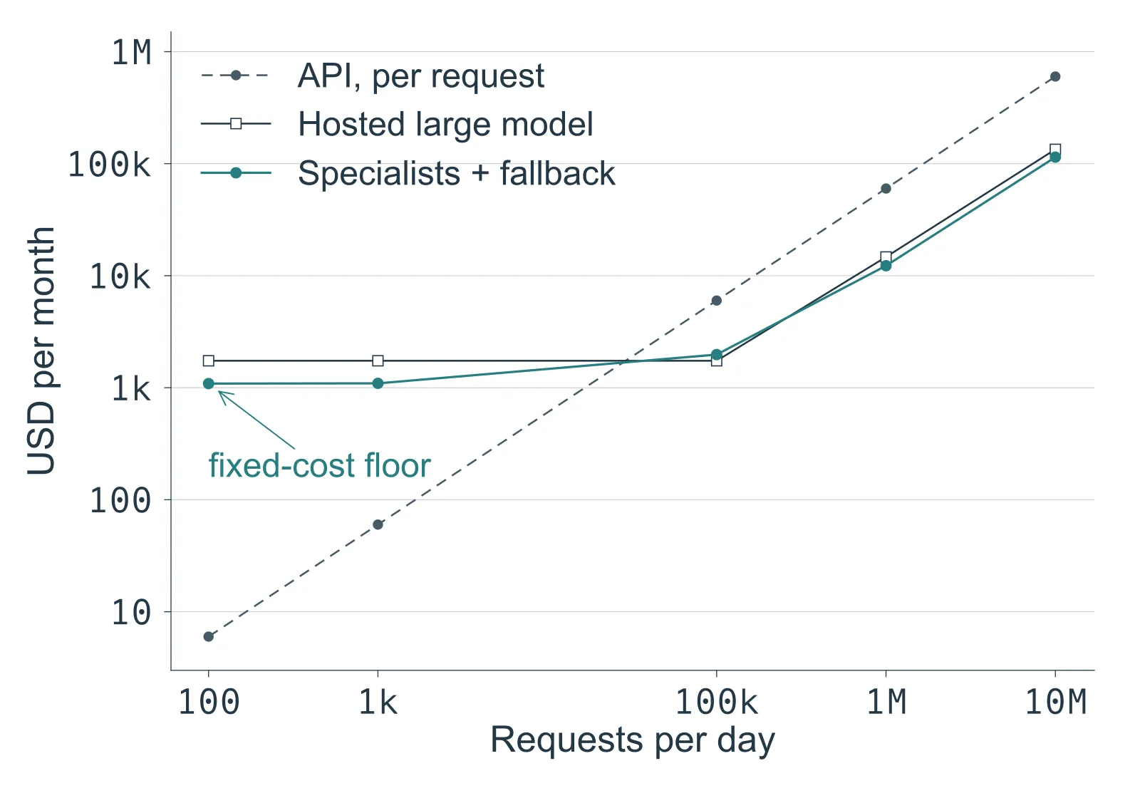
Figure 19.1. Hypothetical USD per month from the saved scenarios, both axes logarithmic. The API line rises with every request; the two hosted lines are flat while one replica suffices and then climb a step at each added replica. The five computed points are joined by straight segments; between them each hosted line is a staircase. The specialists line crosses below the hosted-large line between 100,000 and 1,000,000 requests a day.

Running .venv/bin/python operations.py in the companion directory prints the complete JSON calculation, including these totals, replica counts, and the assumptions label. The committed cost-scenarios.json is a saved copy of that output; the command itself does not write the file. Keeping assumptions beside saved results preserves the basis of the comparison when a table moves into a budget discussion.

Derive break-even, then check the capacity interval

Within a fixed replica count, let F be monthly fixed cost, A the API request cost, and L the local variable request cost. With fallback fraction f, each request saves (1 - f) × A - L compared with sending everything to the API.

Dividing F by a positive saving gives the request count that repays the fixed cost, called the break-even point. A zero or negative saving means additional traffic cannot repay the investment — not at any volume, under the chosen assumptions.

For one specialist unit, hosting costs USD 288, amortized setup costs USD 500, and operations cost USD 300, giving F = USD 1,088. With A = 0.002, f = 0.1, and L = 0, each request saves USD 0.0018.

Save the following as check_break_even.py in the companion directory and run it with python3 check_break_even.py; it imports the companion’s calculator, which needs only the standard library:

from operations import break_even

monthly = break_even(1088, 0.002, 0, 0.1)
max_daily = 5 * 0.5 * 86_400 / 4
print(f"Break-even per month: {monthly:,.0f} requests")
print(f"Break-even per day: {monthly / 30:,.0f} requests")
print(f"One-unit daily limit: {max_daily:,.0f} requests")
print("Nonpositive saving:", break_even(100, 0.001, 0.002, 0.1))

Break-even per month: 604,444 requests
Break-even per day: 20,148 requests
One-unit daily limit: 54,000 requests
Nonpositive saving: None

The crossover at roughly 20,148 daily requests fits below the one-unit limit of 54,000 under the peak and utilization formula. The last line shows a different system whose local variable expense exceeds its available saving, leaving no finite break-even point.

Once traffic requires another replica, F rises and the calculation must be repeated using that new fixed cost. The cost curve is a staircase with variable-cost slopes between steps — each proposed crossover belongs to a particular capacity interval.

Make quality part of the denominator

A cheap request that produces the wrong answer may create more work than an expensive correct one — despite lowering the inference bill. Dividing total cost by acceptable completed requests captures that difference, provided the acceptance rule is fixed before comparing architectures.

Fallback connects answer quality to cost: an invoice specialist can accept easy records cheaply while escalating uncertain ones. We need to measure how often it accepts, how often accepted answers are correct, and what each escalation costs.

A low fallback rate may conceal confident mistakes, while an overly cautious validator may send nearly everything to the expensive path. Coverage and accepted-output error together distinguish an improvement in the model from a change in the gate’s willingness to accept.

Human review adds a term whose size depends on document length, ambiguity, and whether the model supplies a useful candidate. A partially correct extraction can reduce review time even with zero whole-record exact match, but the workflow must establish that saving.

Consequences also differ by field, since an incorrect vendor bank detail can matter more than a missing optional note. An expected-dollar-loss estimate can help a business decision when its assumptions remain visible alongside the underlying technical quality metrics.

Test the assumption most likely to change the decision

The first activity varied fallback because it directly connects the quality decision to the monthly specialist expense. At 100,000 daily requests, each additional ten percentage points of fallback adds 300,000 monthly API calls, costing USD 600.

Fallback fraction	Specialist monthly cost at 100,000/day
10%	USD 1,976
30%	USD 3,176
50%	USD 4,376

These rows change only the fallback input, holding the two specialist units and all other assumptions fixed. In practice, a stricter gate may increase fallback while reducing costly errors, so the economic decision needs both effects.

Capacity uncertainty can matter even more because lower measured throughput brings each additional replica into service at a lower traffic volume. A performance test on the intended serving stack may therefore be more valuable than another training run improving an already sufficient score.

Useful lifetime changes the fixed cost too: spreading USD 3,000 over one month instead of six adds USD 2,500 per month. A rapidly changing schema can erase a saving that depended on keeping the same specialist in service for six months.

The calculator exposes consequences of chosen inputs, making ranges especially useful when measurements are still incomplete or expensive to collect. Find the variable that changes the preferred architecture, then concentrate measurement effort there before refining terms that barely affect the choice.

At very high volume, stage-level load tests and a capacity plan should replace the simplified peak factor and single service rate. The arithmetic remains a useful reconciliation: measured capacity, replica counts, and monthly hours should agree with the bill the team expects.

Count the experiments that did not become releases

The final training runs take seconds or minutes for this book’s fixtures, while developing the specialist also requires datasets, debugging, and review. Reporting only the winning run’s accelerator time omits the effort spent reaching a candidate that passes evaluation.

Track discarded datasets, teacher generations, reviewer hours, and unsuccessful runs alongside the cost of the release that finally ships. If only half the synthetic candidates pass filtering, generation cost per accepted row doubles before review even begins. Near-duplicates can make the cost per new useful decision higher still, despite increasing the accepted row count.

Retraining frequency connects that development work to amortization: a monthly policy change may prevent a specialist from lasting six months. A stable extraction contract can spread the same initial effort over a longer period, lowering its monthly contribution.

The surrounding system can also remove the need for the model, as when a supplier introduces a structured export. A deterministic query builder may replace the reliable SQL subset for similar reasons, changing the economic comparison without another training run.

Exercises

1. Cheap tokens, idle hardware

Why does the API alternative win at one hundred requests per day in the worked scenario?

Answer

Its variable bill is only USD 6 per month, while each hosted arrangement keeps at least one replica provisioned and adds fixed costs. Low per-call compute cost does not offset idle capacity, setup, and operations at that volume.

2. A missing break-even

A local request costs more in variable expense than the API saving after fallback. Can increasing volume make the fixed investment pay back?

Answer

Not under that model. The marginal saving is nonpositive, so each additional request fails to recover the fixed cost. Change the cost, quality, fallback, or capacity assumptions only when evidence supports doing so.

3. The laptop rate

A local evaluation processes one request at a time. Can its requests-per-second number determine production replica count?

Answer

No. It describes that serial inference boundary. Production capacity needs representative concurrency, batching, queueing, stage mix, and latency targets. The local result can inform a measurement plan, but it is not a service load test.

4. A suspicious saving

A specialist’s bill falls after a change that halves fallback calls. Which quality measure must accompany the cost report?

Answer

Measure errors among accepted specialist outputs, along with coverage and end-to-end completion quality. The system may have become more capable, or it may simply be accepting more wrong answers. Cost alone cannot distinguish those outcomes.

Final thoughts

Before buying infrastructure or promising savings, find and measure the assumption that changes the calculator’s answer. Small models can earn an economic advantage when the whole system supports it: a stable task, useful volume, measured capacity, controlled fallback, and operating work we can manage. A low model cost alone does not establish that advantage — the system around it does.

Next: Production Fine-Tuning