When the Small Model Hits Its Limit

A small model’s mistake does not prove that it needs to be larger. The schema may be unclear, the labels may be wrong, the training budget may be too short, or the evaluator may reward the wrong behavior. Scaling before checking those possibilities can buy a more expensive version of the same problem — at a higher price per request.

We can now hold the bookshop schema, execution-based grading, independent Python oracles, and dataset fixed while comparing model sizes. That gives us a specific question: does more base-model capacity change the same twenty-four answers under the same adaptation recipe?

We need a candidate that meets the application’s quality gate at a latency, memory, storage, and operating cost we can accept. A larger model may be the right choice — it earns that place by handling the workload, rather than by having the highest parameter count.

Run against: Qwen3-0.6B, Qwen3-1.7B, Qwen3-4B, and Qwen3-8B at revisions in scaling-models.json; Transformers 4.56.2, PEFT 0.17.1, bitsandbytes 0.50.2, PyTorch 2.8.0, NF4 double quantization with float32 compute, Apple M1 Ultra/MPS.

Not run. Multi-seed uncertainty, per-size hyperparameter tuning, equal-compute training, CUDA comparisons, production concurrency, and independent compositional SQL generalization are outside this study.

All sizes see the same seventy-two training rows and twenty-four test rows. Those rows share twelve query families, so the comparison measures a narrow adaptation problem rather than a universal reasoning limit.

Distinguish a task limit from a model limit

A model cannot infer a business rule that the task never defines. If “revenue” might include tax or refunds but the schema contains neither, the task must first state what its available fields mean. A larger model would face the same missing definition — just as Chapter 15’s evaluator needed one before it could grade queries.

Preprocessing can create a similar problem by removing information the model needs. If a long schema is truncated before the relevant table, more examples may teach guessing instead of using the source. Inspect the encoded input and labels together: a correct query graded against a flawed oracle can make a capable model appear weak.

The remaining question is whether the training recipe taught the distinction sufficiently. A short run may leave useful behavior unlearned, while an aggressive learning rate may damage behavior the base already had. After checking the task, input, labels and optimization, comparing stronger bases becomes a focused experiment rather than a response to any disappointing score.

Keep the comparison controlled and its question narrow

The four arms use Qwen3 sizes labeled 0.6B, 1.7B, 4B, and 8B, with each model and tokenizer pinned to an exact repository revision. The companion downloads those revisions from scaling-models.json, so another run starts from the same checkpoints rather than a moving branch.

Each arm begins with its own base checkpoint and receives the same policy, schema, training and test data, decoder, sequence budget, seed, and adapter targets. It first receives a zero-shot evaluation in its quantized state, then trains for one epoch over seventy-two rows at batch size one. The final adapter is evaluated without demonstrations — and no adapter is continued into the next size.

Controlled choice	Value
Training examples	72
Test examples	24
Database fixtures	2
Optimizer steps	72
Adapter rank and alpha	8 and 16
Adapter targets	Query and value projections
Learning rate	0.0002
Weight decay	0.01
Sequence width	256 tokens
Decoder	Greedy, thinking disabled, at most 160 new tokens

The models have different parameter shapes within the family, so rank eight does not fix the number of trainable adapter parameters. Larger projections and more layers can make the adapter itself larger — the resource table records that difference alongside training time.

Equal steps hold example exposure constant, while each larger-model step performs more work. This is a comparison under one adaptation recipe, rather than each size’s best possible tuning or an equal-compute allocation. An equal-time study would answer a different question and might give larger models fewer steps.

Compare like quantization with like quantization

All four SQL arms use NF4 storage with double quantization and float32 computation, reusing the QLoRA setup from Chapter 15. The runner loads and quantizes on CPU before moving to MPS; both base and adapted evaluations use that representation for each size. The comparison therefore keeps quantization consistent while changing the model and its learned adapter.

Four-bit storage still leaves embeddings, normalization, adapters, activations, optimizer state, and working buffers in other representations. Chapter 9’s memory distinction applies here: half a byte per nominal parameter is only part of the allocation, so the recorded counters matter more than that shortcut.

The installed bitsandbytes path supports this pinned setup; the Transformers bitsandbytes documentation explains its configuration concepts. All models also use the non-thinking chat-template path described in the Qwen3 model card, keeping the generation budget focused on the requested query.

Record the resources that a release actually needs

Training time covers the optimization loop, excluding download, loading, quantization, artifact saving, and evaluation; model-load time is recorded separately. The saved artifact contains adapter and tokenizer files, while the frozen base remains in its cache. Its directory size therefore measures the incremental package rather than everything a deployment needs.

MPS allocated and driver memory are snapshots taken after training; process peak RSS is the operating system’s peak resident-memory measurement for the process. These counters describe different scopes on unified-memory hardware, and none establishes peak device allocation. The true MPS peak field remains null — preserving the missing measurement instead of substituting a convenient snapshot.

Latency covers warmed serial calls: tokenization, generation, decoding, and device synchronization, with loading and grading excluded. P50 is the median, and P95 is the 95th percentile, describing the slower end of the sample. Serial requests per second divides the request count by total inference time, so it uses the mean rather than the median.

The models use the device sequentially on an ordinary desktop with background activity, including downloads and manuscript tooling. Those conditions make close timing differences worth repeating before they determine a deployment choice — the table records these runs, not a concurrent service benchmark.

Quality measure	0.6B	1.7B	4B	8B
Base execution-correct	1/24	17/24	21/24	23/24
Base valid	18/24	21/24	24/24	24/24
Adapter execution-correct	22/24	24/24	24/24	24/24
Adapter valid	24/24	24/24	24/24	24/24

Resource measure	0.6B	1.7B	4B	8B
Training seconds	22.33	47.24	127.70	217.01
Load seconds	3.04	7.45	13.68	17.75
Adapter + tokenizer MiB	19.54	21.29	26.42	29.80
MPS allocated snapshot MiB	911.70	2037.80	3444.93	8370.07
MPS driver snapshot MiB	4476.86	5511.94	14071.30	17951.16
Process peak RSS MiB	3385.38	5986.53	7995.80	10698.31
Adapter P50 inference ms	2063.2	4348.7	12436.7	23248.0
Adapter P95 inference ms	3552.5	6280.8	21297.8	40099.3
Adapter serial requests/s	0.516	0.231	0.085	0.046
Trainable adapter parameters	1,146,880	1,605,632	2,949,120	3,833,856

Read improvement as changed answers

Chapter 15 left the 0.6B adapter with two anti-join failures. Before interpreting the larger scores, compare one of those saved answers with the 1.7B answer on the same request. From the companion directory, save this as compare_sql_sizes.py and run python3 compare_sql_sizes.py; it uses only the standard library and downloads no models:

import json
from pathlib import Path

case_id = "sql-test-07-anti_join"
for size in ("0.6B", "1.7B"):
    path = Path(f"runs/sql-{size}-v1/test-zero.jsonl")
    rows = [json.loads(line) for line in path.read_text().splitlines()]
    row = next(r for r in rows if r["id"] == case_id)
    print(size, "valid:", row["valid"], "exact:", row["exact"])
    print(row["raw"])

0.6B valid: True exact: False
SELECT id FROM books WHERE NOT EXISTS (SELECT 1 FROM sales WHERE sales.book_id=id) ORDER BY id
1.7B valid: True exact: True
SELECT id FROM books WHERE id NOT IN (SELECT book_id FROM sales) ORDER BY id

The smaller query contains the inner-scope id mistake already traced in Chapter 15. The larger query instead collects sold book IDs and keeps catalog IDs outside that collection — another way to express absence in this fixture. The 4B and 8B adapters write a third form, the reference’s own correlated NOT EXISTS with the b and s aliases, so the three passing sizes reach the answer two different ways. Only execution-based grading can call all of them correct; a string comparison with the reference would have failed the 1.7B answer that Chapter 15’s evaluator rightly accepts.

Both answers are executable, so this change repairs the requested relationship rather than merely removing Markdown or fixing syntax. The two test variants receive the same query at each size, accounting for the increase from twenty-two to twenty-four correct answers. The per-family table makes that location visible:

Query family	0.6B	1.7B	4B	8B
select	2/2	2/2	2/2	2/2
filter	2/2	2/2	2/2	2/2
category	2/2	2/2	2/2	2/2
sum	2/2	2/2	2/2	2/2
join	2/2	2/2	2/2	2/2
revenue	2/2	2/2	2/2	2/2
group	2/2	2/2	2/2	2/2
having	2/2	2/2	2/2	2/2
cte	2/2	2/2	2/2	2/2
window	2/2	2/2	2/2	2/2
anti_join	0/2	2/2	2/2	2/2
average	2/2	2/2	2/2	2/2

Each family has only two requests, so its possible scores are zero, fifty, or one hundred percent. A perfect row means those two requests pass on both fixtures, and shared query families leave familiar SQL patterns available to every model. The table identifies the repaired behavior — it cannot tell us which internal capability produced it.

The same inspection should look for regressions, because a larger total can hide damage to previously correct requests. If added capacity mainly fixes formatting, a prompt or constrained decoder may deserve comparison; if it repairs a relational distinction, targeted examples remain a useful alternative experiment.

Choose the smallest model that clears a declared gate

Before test inspection, the study declares an illustrative gate: at least ninety percent execution exact match and one hundred percent valid queries. On twenty-four cases, that requires at least twenty-two correct answers and no rejected queries. The 0.6B adapter clears both conditions — so a higher score alone does not require choosing a larger model.

A real application needs a gate tied to consequences, supported query families, and any review path; ninety percent is only this teaching comparison’s threshold. If every supported answer must pass, or a crucial family remains wrong, the requirement can justify moving beyond the smallest eligible candidate.

When no candidate passes, changing the threshold should be an explicit product decision with recorded consequences. Diagnosing the failures and evaluating a revised candidate preserves the meaning of the original comparison — quietly lowering the gate after seeing its results does not.

Work through a capacity decision with two constraints

Suppose an internal reporting tool adopts that illustrative quality gate and requires warmed median model inference below five seconds on this machine. The 0.6B median is about 2.06 seconds, and the 1.7B median about 4.35 seconds, so both remain eligible. The 4B adapter’s roughly 12.44 seconds excludes it despite its perfect test score.

Now require all twenty-four answers to be correct while keeping the five-second median limit. The 0.6B candidate drops out, leaving 1.7B as the smallest eligible size — the choice changes because the requirement changed. These are hypothetical product limits applied to recorded measurements, making the decision inspectable without claiming that five seconds suits every workflow.

A five-second P95 limit would change the answer again, because the 1.7B run’s P95 is about 6.28 seconds. None of these candidates then satisfies both the perfect-test requirement and that tail-latency constraint. The product must specify which part of the response-time distribution it promises, rather than treating a median and a P95 as interchangeable.

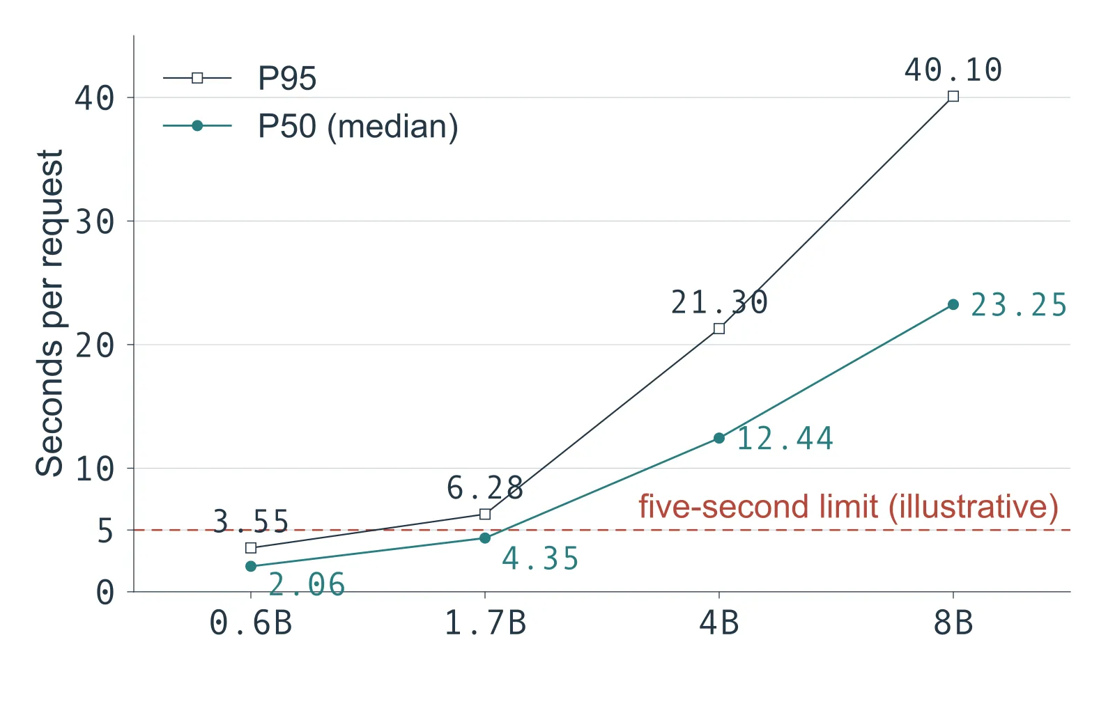
Figure 16.1. Warmed serial inference on the author’s machine, from the resource table. Under a five-second median limit the 0.6B and 1.7B adapters are eligible and the two larger ones are not; under a five-second P95 limit only 0.6B remains, and it misses two answers. Timings come from one run each on an ordinary desktop.

A user-facing deadline also includes routing, data access, validation, queueing, and fallback. Adding component medians generally does not recover the assembled system’s median, especially when routes and request lengths differ; Chapter 18 brings those stages together so the complete path can be measured.

Memory fit requires exercising the intended lifecycle, including loading, temporary buffers, activations, and concurrent work. Use the table’s named counters to compare the recorded runs, then measure whether the candidate actually fits that lifecycle. Similarly, deployment storage includes the base cache as well as the adapter: specialists sharing a base revision may share files, while different bases require separate weights.

Keep quality, latency boundary, memory scope, and complete deployment artifacts in separate worksheet columns. That makes the binding constraint visible and includes the files needed for recovery, which a single undocumented “efficiency score” could hide.

Recognize diminishing returns without claiming a law

Moving from 0.6B to 1.7B fixes the remaining two test answers, leaving no additional score for the larger adapters to gain. The test has reached its ceiling — latency and resource differences remain visible. A broader workload could still distinguish the models — this one cannot rank quality after every case passes.

A more demanding reserve could introduce new compositions, schemas, ambiguous requests, unsupported operations, and independently authored wording. Define its scope before using results to select a candidate, so extending evaluation answers a product question instead of searching for cases that favor one size.

Difficulty alone is not the goal: a test dominated by hard requests can overlook an easy, high-volume subset that specialists could serve reliably. Report the intended supported slices and their escalation paths, then choose capacity for that scope rather than requiring one model to handle every request.

Diagnose a plateau before buying more hardware

The paired predictions also guide the next experiment when several sizes plateau. Shared semantic errors send us back to the task and labels; an error confined to the smallest model makes capacity more plausible. Failures that vary across repeated runs instead point toward optimization instability or small-sample noise.

Each adapted model should also be compared with its own base, because deterioration after training suggests a problem with adaptation. More parameters do not protect a model from learning a narrow or inconsistent target distribution, even when its initial capability is strong.

The next experiment should test one suspected cause: add targeted examples, extend the training budget, alter adapter scope, or clarify the schema. A control and fresh reserve help interpret the result, whereas changing everything together obscures what repaired the error. The economical choice can then reflect both serving resources and the review work that remaining mistakes create.

Reproduce the sweep without hiding downloads

The saved-answer activity checks what the recorded models returned; repeating training asks whether the recipe produces comparable behavior in another run. Use the frozen environment and the following commands when you want that second experiment. The download script reads pinned revisions from scaling-models.json; the larger checkpoints require substantial cache space and download time beyond the table’s training seconds.

.venv/bin/python download_scaling.py

for size in 0.6B 1.7B 4B 8B; do
  .venv/bin/python specialist_run.py \
    --task sql --size "$size" --quant --before --train \
    --epochs 1 --batch 1 --output "runs/local-sql-sweep-$size"
done

The loop runs models serially on MPS, with a separate adapter and output directory for each size; every destination must be absent. Its local-sql-sweep prefix separates this comparison from Chapter 15’s local-sql-0.6B run. Choose another local prefix when repeating the sweep, keeping earlier results available for comparison.

The runner prints progress during training and writes predictions, losses, configuration and metrics beneath each destination. The same result format is available in the frozen runs, so save this as read_sql_sweep.py and run python3 read_sql_sweep.py to inspect the recorded counts without training:

import json
from pathlib import Path

for size in ("0.6B", "1.7B", "4B", "8B"):
    path = Path(f"runs/sql-{size}-v1/results.json")
    run = json.loads(path.read_text())
    score = run["metrics"]["test-zero"]
    correct = round(score["exact_match"] * score["n"])
    print(size, "steps:", run["optimizer_steps"],
          "correct:", f"{correct}/{score['n']}")

0.6B steps: 72 correct: 22/24
1.7B steps: 72 correct: 24/24
4B steps: 72 correct: 24/24
8B steps: 72 correct: 24/24

To inspect your new run, change the script’s path to runs/local-sql-sweep-{size}/results.json, matching any alternative prefix you used. Its counts may differ from the frozen comparison.

Regrading saved SQL checks the evaluator and reporting arithmetic; retraining also tests the learning process. Neither substitutes for evaluating a new workload, but each answers a useful, distinct reproduction question.

Exercises

1. Equal steps, unequal work

All four models train for seventy-two steps. Does this make the sweep equal-compute?

Answer

No. Larger models do more work per step, and rank-eight adapters can contain different numbers of parameters at different sizes. The study holds the recipe and example exposure constant. An equal-time or equal-cost study would need a different budget allocation.

2. A test ceiling

Two model sizes both answer all twenty-four cases correctly. What can be concluded about their relative capability?

Answer

They tie on this test under this recipe. The test cannot reveal additional quality beyond its ceiling. Compare measured resources for this workload, and use a broader independent reserve before making claims about more difficult tasks.

3. A memory column

The runner records MPS allocation after training and process peak RSS. Can either be labeled “peak GPU memory”?

Answer

No. The first is a device allocation snapshot, and the second is process resident memory. Neither establishes the true peak device allocation. Preserve the measurement names and leave an unavailable peak as unavailable.

4. A small model that passes

The 0.6B adapter meets the declared quality and validity gate, while a larger model scores better but takes longer. Which model must be selected?

Answer

There is no universal requirement to select the higher score. Under the declared gate, the smaller model is eligible and may be preferable. A stricter quality requirement or different workload could justify the larger one. Make that decision from the application’s constraints, not parameter count alone.

Final thoughts

Once the task and evaluator are clear, scaling can help us choose the capacity we actually need. The smallest candidate may already be sufficient. If we choose more parameters, we should be able to name the needed behavior they buy us.

Next: Prompt, Retrieve, Fine-Tune, or Scale?