How Much Training Data Do You Need?

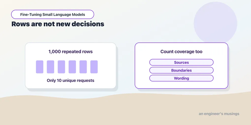
A file with one thousand rows can contain only ten ideas. Repeating each request a hundred times changes how often the optimizer sees it, but it does not teach the router a new boundary. That makes “How many examples do I need?” a question about coverage and optimization rather than about file length.

The bookshop study trains LoRA adapters with 10, 50, 100, 500, 1,000 and 2,000 rows. Each size is a separate experimental arm: a training run starting again from the same base checkpoint. A control of 1,000 rows made from only ten unique requests runs beside them, exposing what repetition buys. The measured curve relates training-row count to performance under this recipe. Its horizontal axis counts rows, which need not count distinct ideas — and one failure in the results makes that distinction concrete.

We want the experiment to say what to collect next. We take progressively longer portions from the start of the same training file, called prefixes. They are nested because each contains the smaller collection, and balanced because each keeps equal counts across labels. More paraphrases may add little when a small collection already covers the recurring decisions. When a costly boundary is missing, ten chosen examples can teach more than a large batch of familiar wording.

Run against: PEFT 0.17.1, PyTorch 2.8.0, Transformers 4.56.2; pinned Qwen3-0.6B, rank-eight query/value LoRA, float32 Apple M1 Ultra/MPS, seed 42, dataset router-v2, fixed plan training-v2. The per-step losses quoted are the recorded sweep runs’ loss.jsonl files and the errors are their saved test predictions.

Not run. Multiple-seed confidence intervals, independently authored evaluation, representative traffic, a fixed-step sweep, and an annotation-quality ablation are outside this study.

Decide what the curve is allowed to answer

A learning curve relates training data to measured performance, and it is tempting to read it as a property of the model: “this model needs five hundred examples.” In fact the curve depends on the task, the label quality, the selection order, the training budget, the hyperparameters and the evaluation distribution. The router’s label space is small, the policy is stated at inference, and the model already has general language ability. That makes this experiment unlike learning a new language or inferring an unstated business rule.

Example quality moves the curve as much as count. A collection covering missing operands, source precedence, quoted instructions and clarification can teach more than an equally sized collection of obvious stock lookups. Size has meaning only beside a description of what was added. Our study asks the narrower, reproducible question: under two epochs of the declared LoRA recipe, how do these nested balanced prefixes perform on the same reserved template families? The final checkpoint of every arm is evaluated without the test choosing an epoch or a learning rate. Once the results are inspected, this test joins the accumulated development knowledge, and a round designed around its failures needs a new final reserve.

Build nested collections with visible composition

Nested collections make the comparison interpretable, because the ten-row set is inside the fifty-row set, which is inside the hundred-row set. An improvement cannot be explained by the larger set having dropped a difficult example the smaller one contained.

The core is interleaved by class, so every prefix is balanced. The first 150 rows are the individually authored requests from Chapter 6, and larger prefixes add deterministic variants from forty training templates.

Training rows	Per class	Individually authored rows	Template-derived rows
10	2	10	0
50	10	50	0
100	20	100	0
500	100	150	350
1,000	200	150	850
2,000	400	150	1,850

The composition is deliberately visible — the jump from one hundred to five hundred rows changes both the count and the source mix. Larger sets hold more surface variation but not proportionally more routing concepts, so a plateau can reflect template redundancy as much as the model’s data efficiency.

The poor-data control repeats the first ten balanced requests one hundred times: 1,000 rows, ten unique texts, labels intact. Its weakness is narrow coverage and repetition, not corruption. The experiment can therefore compare a thousand repeated correct rows with a hundred distinct ones, but it cannot say how a thousand mislabeled requests compare with a hundred correct ones.

Start every arm from the same base

A size sweep must not quietly become continued training. If the fifty-row run started from the ten-row adapter, it would inherit that optimization, the hundred-row run would inherit both, and the displayed size would no longer describe the history. Each companion invocation therefore loads the pinned base and initializes a fresh rank-eight adapter. The seed, target modules, learning rate, batch size, weight decay, clipping and decoder are fixed; only the selected rows and the resulting number of batches change.

The companion’s driver script runs each size independently: the loop starts a new training process for each collection. The control is one more invocation with a --poor flag. It repeats the small collection rather than introducing incorrect labels. These commands use the prepared training environment and new output directories; the saved losses and results below also support reading the experiment without rerunning the sweep:

for size in 10 50 100 500 1000 2000; do
  .venv/bin/python train_router.py \
    --mode lora --size "$size" --epochs 2 \
    --output "runs/local-size-$size" --evaluate test
done
.venv/bin/python train_router.py \
  --mode lora --size 1000 --poor --epochs 2 \
  --output runs/local-size-poor1000 --evaluate test

The runner stores the selected size and the unique-text count in each run’s metadata, so a thousand repeated rows cannot be mistaken for a thousand unique requests. The manifest and runner hashes identify the data construction and code used. A fixed seed gives the arms a shared starting condition without making their trajectories identical — different sizes produce different shuffled sequences and different numbers of updates. Keeping the base fixed also keeps model size out of the study. A larger checkpoint is a separate axis, and mixing the two in one small table would make their effects impossible to separate.

Count the optimization budget beside the rows

Two epochs means each row is presented twice, but larger datasets produce more optimizer updates. With batch size four and the final batch retained, divide the row count by four and round upward to count the batches in a pass. This upward rounding is called the ceiling. Twice that count gives the optimizer steps. The table also counts example presentations: every occasion on which a row is shown, including its return in the next epoch:

Rows	Epochs	Optimizer steps	Example presentations
10	2	6	20
50	2	26	100
100	2	50	200
500	2	250	1,000
1,000	2	500	2,000
2,000	2	1,000	4,000

The ten-row model receives six updates, so if it performs poorly, limited optimization is part of the explanation. The two-thousand-row model receives a thousand, so its result combines broader exposure with a far larger budget. This is a fixed-epoch curve, not a fixed-compute one. Fixed epochs ask what happens when a normal pass-based recipe grows with the data. Fixed steps ask how different collections use the same number of updates, at the cost of repeating small collections many times and perhaps never fully seeing large ones. Either design is legitimate if it reports its sampling policy. Here the repeated-data arm shares its row count and step budget with the ordinary thousand-row arm, which is what lets the two isolate the value of coverage under this recipe.

Run the sweep and watch the smallest arm

The ten-row arm is the one to watch, because it is the only arm that fails. Its whole training run is six optimizer steps. This is its complete loss.jsonl, with the losses rounded to three decimals:

{"step": 1, "epoch": 0, "loss": 0.827}
{"step": 2, "epoch": 0, "loss": 0.491}
{"step": 3, "epoch": 0, "loss": 0.288}
{"step": 4, "epoch": 1, "loss": 0.477}
{"step": 5, "epoch": 1, "loss": 0.023}
{"step": 6, "epoch": 1, "loss": 0.013}

Six updates, 2.95 seconds — and a loss that has clearly started to fall. On the test it scores 90%: five errors, and all five are the same thing. The test family test-DOCUMENT-1, whose five rows are test-DOCUMENT-01-000 to 004, asks in five slot variants, “An uploaded spreadsheet already contains the answer. Which row names Alex 1?” — and the ten-row adapter sends every variant to DATABASE. The required source is the supplied spreadsheet, so the policy calls for DOCUMENT. This six-update recipe has not learned to route that family correctly. The error alone cannot tell us whether more examples or more optimization would help, or whether the phrase “which row” influenced the choice. The repeated-data control below tests what happens with more updates on the same ten requests.

The fifty-row arm — the same ten rows and forty more — gets the family right. Its 26 steps start at 0.621, are at 0.049 by the third step, and end at 0.001 and 0.000 — with step 24 back up at 0.729, the usual noisy batch. Five row-level gains between the two arms are therefore one newly handled wording pattern, not five independent discoveries. That is the pattern for reading every other point on this curve: count families, not rows.

The repeated-data control is the other run worth opening. Its 500 steps begin at 0.598, 1.051 and 0.516, and its last three are 0.000, 0.000 and 0.000. Ten requests seen a hundred times each leave the model with nothing left to learn from them. The 2,000-row arm is at 0.00004 by step 500 of its thousand.

Read the measured curve without smoothing away its limits

Rows	Unique texts	Steps	Accuracy	Macro-F1	Training s
10	10	6	90%	0.893	2.95
50	50	26	100%	1.000	13.43
100	100	50	100%	1.000	26.40
500	500	250	100%	1.000	131.29
1000	1,000	500	100%	1.000	262.92
2000	2,000	1000	100%	1.000	525.87
poor1000	10	500	100%	1.000	262.70

poor1000 is the repeated-data control, and every invalid-output count is zero.

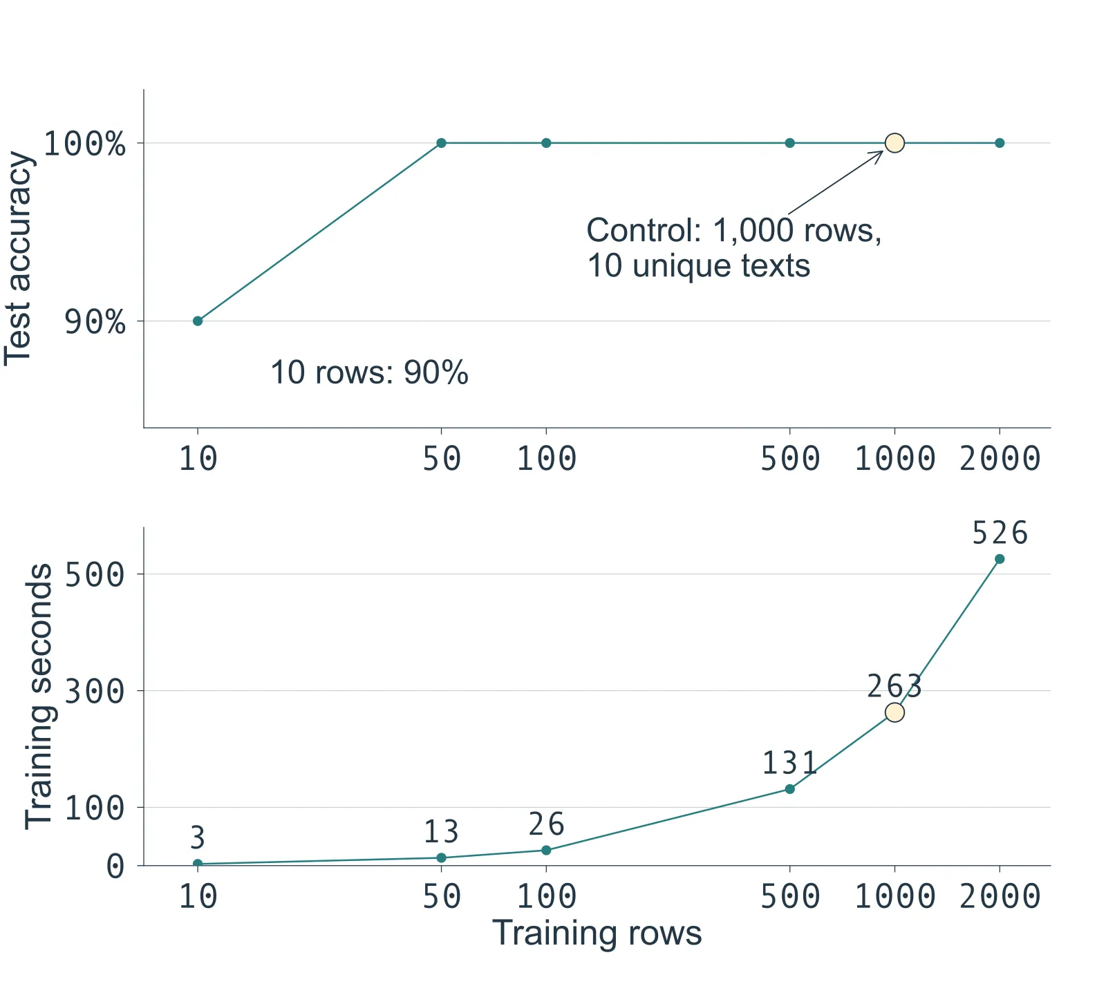
Figure 10.1. Every point is one recorded arm; the amber point is the repeated-data control, which shares the thousand-row arm’s step budget. Accuracy reaches the test’s ceiling at fifty rows and stays there while training time keeps climbing. The horizontal axis is logarithmic.

The curve reaches 100% at fifty rows and stays there through two thousand. The repeated-data control reaches 100% too, from the same ten requests that scored 90% after two epochs: more optimization on the same ten texts changed the outcome without adding a request. The hundred-request authored prefix and the thousand-row repeated control therefore tie on this fixture. The prefix gets there in 50 updates and 26.40 seconds, the control in 500 updates and 262.70 seconds — an observed cost difference at the test’s ceiling, not proof that the two generalize equally or that repeated data would survive deployment.

There is no measured quality gain from the larger prefixes on this test, while training time rises from 13.43 seconds at fifty rows to 525.87 at two thousand. The honest next investment is a stronger evaluation, followed by targeted collection if it exposes missing behavior. Reporting that is more useful than drawing a steadily improving curve the data does not contain. Each point rests on fifty test requests from ten reserved families, so the effective diversity of the judgment is far smaller than “fifty held-out examples” suggests.

A curve of this kind need not be monotonic: adding data need not always hold or improve the score. A rising region shows the larger prescribed recipe doing better on these requests; a flat region shows no observed gain. A drop can reflect overfitting, the added data’s composition, optimization effects or the sensitivity of one trajectory. The table alone cannot distinguish those causes. The saved raw predictions let us examine what changed. If a larger arm gains three cases and loses three others, accuracy holds still while behavior changes, hiding a possibly costly regression. Fitting a smooth saturation function to six single-seed points would give a precise “required sample count” without sufficient evidence.

Distinguish diminishing returns from a weak test

Suppose scores stop improving after a hundred rows. That can mean the training distribution has little left to teach, or that the test is too easy or too narrow to detect progress. The useful follow-up asks where the model is expected to generalize: long requests, conversational references, source conflicts, misspellings, ambiguous attachments. Adding those to a development collection finds missing behavior, and a separate reserve then judges the revised candidate.

More evaluation data can be worth more than more training data when uncertainty dominates the decision. If two candidates differ on one of fifty templated rows, a day spent generating another thousand training variants will not say which is safer to deploy. A carefully sampled evaluation collection will. Error cost shapes the answer too. Fixing a rare route that triggers an expensive external lookup may matter more than polishing several harmless wording edits, and a single accuracy number weighs every row the same. A representative traffic sample and a boundary stress set answer complementary questions, and keeping them separate stops a deliberately hard test from being mistaken for the daily error rate.

Make repetition an explicit control

Repeated requests are not useless. Additional presentations can let the optimizer settle a pattern a few updates did not, and repetition is implicit in every multi-epoch run; the problem is calling repetition new evidence. The thousand-row control makes the distinction visible: ten balanced, consistently labeled requests with many chances to be learned. Had it performed worse than the broad collection, that would have supported the value of coverage under this recipe. Performing the same, as it did, says the reserved test is too narrow to expose the difference, or that those ten patterns already support its decisions.

Label noise is a separate experiment, and this study keeps labels intact so that repetition stays the one stated weakness. Near-duplicates sit between exact repetition and genuinely new scenarios. A template with a different product title may improve robustness to surface variation, but it rarely carries as much policy information as a request that changes the required source. That is why a data report should count families as well as rows.

Spend annotation effort on the next decision

After a first curve, data work can be targeted. Group the errors by the policy distinction they violate: missing arithmetic inputs form one group, a supplied document confused with current external evidence another. The groups say both what examples to write and whether the policy itself is incomplete. The ten-row arm’s family is a worked case — a supplied document that reads like a records question.

A useful new batch puts positive and contrasting examples around each boundary. If a router reaches for DATABASE whenever the word appears, add general explanations about databases beside true record lookups. If it reaches for WEB for anything that sounds current, contrast a live lookup with a date quoted in an attached document. The new examples should vary more than nouns — sentence structure, implied source, negative phrasing, the position of the decisive clause. They still need review, because adversarially complicated wording can become ambiguous under the policy, and an unclear example teaches uncertainty rather than robustness.

Failure-driven collection also changes the status of the examples that motivated it. Those inspected failures become development evidence. A later final test needs independent cases that assess the revised boundary without repeating its wording; otherwise the loop rewards memorizing the evaluator’s complaints. This is where a larger synthetic-generation pipeline helps, provided generation is followed by validation, deduplication and provenance checks. Chapter 11 builds that pipeline around known source records and measured student behavior.

Inspect the marginal result as a paired decision

A paired comparison follows the same request through both candidates and records whether each answer is correct. The resulting two-by-two table groups requests both get right, requests both get wrong, gains and regressions. A gain is a corrected earlier error; a regression is a previously correct route that becomes wrong. The balance of gains and regressions explains the net accuracy change; the requests themselves show which decisions improved or worsened.

For an illustrative fifty-case comparison, suppose thirty-eight requests are right under both models, five are wrong under both, five improve and two regress. The first candidate gets forty right and the second forty-three — a headline gain of six points — while seven decisions changed and two became worse. Those counts are arithmetic, not another measured router result. They show why a curve point should keep its predictions: if both regressions concern missing operands and send private-record requests to a calculator, the larger model may still violate the requirement that matters most.

A minimum acceptable score can guide selection when it is paired with explicit boundary requirements, such as no observed unauthorized-source routing on a dedicated stress set. That is a measured acceptance condition on a finite set, not a proof. Choosing the smallest candidate that clears meaningful requirements is often better than maximizing a noisy score, because it reduces training and maintenance effort while keeping the behavior the application needs. The requirements have to be written down before the ranking is inspected if they are to act as a real decision rule.

Preserve the decision, not just the winning number

A useful report keeps every arm, including the regressions and invalid outputs, because deleting a disappointing run makes the selected result look more inevitable than it was. The fixed plan and output directories keep the comparison auditable. It keeps the training cost too. Two candidates with similar routing quality can differ greatly in update count, wall time and collection effort, and if the larger set adds little on a meaningful evaluation, the smaller candidate is easier to reproduce and maintain.

Training wall time is only one cost. Writing a new policy distinction, reviewing ambiguous examples and adjudicating disagreements can dominate the effort for a small model. Generated rows that are cheap to produce can still be expensive to validate. A collection log that records accepted rows, rejected rows, unique scenario families, reviewer time and the reasons for rejection makes it possible to ask whether the last batch bought coverage. Counting accepted rows alone hides a generator that produces mostly unusable requests. This fixture records construction, not dollar cost; operational data would need a new provenance record and a new cost analysis. The result should end in a specific next action — collect a missing boundary, strengthen the test, repeat seeds, try a fixed-step comparison, or keep the current adapter. Before “generate more data” is chosen, the new information those examples are to supply should be named.

Exercises

1. Interpret two thousand rows

A dataset has 2,000 rows created from forty templates. Why should its report include both numbers?

Answer

Rows describe the optimizer’s available examples. Templates describe an important source of correlation and limited structural diversity. Two thousand surface variants are not equivalent to two thousand independently sourced requests, even when every text is unique.

2. Identify the compute confound

A hundred-row arm and a thousand-row arm both train for two epochs at batch size four. How many updates do they receive, and what does that change in the interpretation?

Answer

They receive 50 and 500 updates. The larger arm has more data and ten times as many optimization steps. Its result belongs to a fixed-epoch recipe; it does not isolate data size under equal compute.

3. Explain a flat accuracy curve

Two models each get 45 of 50 cases correct. One fixes three earlier errors and introduces three new errors. Did nothing change?

Answer

Behavior changed on six cases even though net accuracy did not. Paired predictions and per-class metrics reveal those changes. Their operational importance depends on the routes and error costs involved.

4. Choose the next investment

All six sizes score almost perfectly on ten test families, but production requests are longer and more ambiguous. Should the next step be declaring the minimum sufficient dataset size?

Answer

No. The evaluation does not cover the deployment conditions. A stronger, independently reviewed evaluation set should precede a sufficiency claim. The current result only establishes performance on the narrow reserved families.

Final thoughts

I would choose the next examples by the decisions they add, then use a measured curve to see whether the model learns them. Row count is a useful bookkeeping field. Coverage, label consistency, and an evaluation that can still surprise us decide whether collecting those rows was worthwhile — and the ten-row arm’s one failing family is the kind of surprise to go looking for.

Next: Synthetic Data Generation