Files to Answers
A complete workflow on 7.4 million rows of real, dirty data nobody cleaned for you — queried over HTTP before it was downloaded, including the file named for April 2019 that contains trips from 2008 and 2033.
Every example so far has been chosen to make a point. This one is not.
The dataset is a public Parquet file of New York taxi trips — 7.4 million rows, produced by a regulator, cleaned by nobody. It is on a web server. There is no schema documentation, no data dictionary, and no promise that its contents match its filename.
What follows is the actual sequence of a real investigation, in the order it happened. Look at it before downloading it. Find out how much of it is wrong. Build the analysis on what survives, and stop querying the network once you know what you are asking. Every number below came out of the run.
Everything here was run against DuckDB 1.5.5.
Look before you download
select count(*) from 'https://blobs.duckdb.org/data/taxi_2019_04.parquet';7433139[1622 ms]Seven and a half million rows, counted over the public internet, in under two seconds. No download, no INSTALL, no LOAD. Chapter 9 explains the missing step: DuckDB saw https://, autoloaded httpfs, and read the Parquet footer over a range request. The row count is in the metadata, so almost none of the file was fetched.
Next, the schema, which is the only documentation that exists:
describe select * from 'https://blobs.duckdb.org/data/taxi_2019_04.parquet';vendor_id VARCHAR
pickup_at TIMESTAMP
dropoff_at TIMESTAMP
passenger_count TINYINT
trip_distance FLOAT
rate_code_id VARCHAR
store_and_fwd_flag VARCHAR
pickup_location_id INTEGER
dropoff_location_id INTEGER
payment_type VARCHAR
fare_amount FLOAT
…
total_amount FLOAT
congestion_surcharge FLOATEighteen columns, properly typed — timestamps are timestamps, not strings — because Parquet carries its schema and there was nothing to infer. That is chapter 4’s argument arriving as a convenience rather than a lecture.
Two queries in, we know the size and the shape, and nothing is on the disk.
Find out what is wrong with it
The file is called taxi_2019_04.parquet. Check the claim in its name:
select min(pickup_at), max(pickup_at)
from 'https://blobs.duckdb.org/data/taxi_2019_04.parquet';
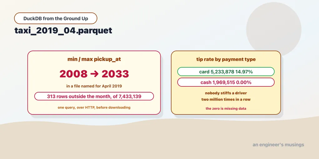
(2008-08-08 09:13:28, 2033-04-27 13:08:32)2008 to 2033. In a file named for April 2019.
This is the moment the whole book is for. That query took ten seconds over HTTP and it invalidated any analysis that had assumed the filename. Nobody would have caught it downstream — a monthly average is still a number when the month is wrong.
How bad is it?
select count(*) from … where pickup_at < '2019-04-01' or pickup_at >= '2019-05-01';313select date_trunc('year', pickup_at) yr, count(*) n from … group by 1 order by 1;(2008-01-01, 18)
(2009-01-01, 49)
(2019-01-01, 243)
(2033-01-01, 3)Three hundred and thirteen rows out of 7.4 million — four thousandths of a percent. Small enough to be invisible in any aggregate, large enough to ruin a min(), a max(), or any chart with a time axis. Three of them are in 2033.
Keep going, because bad timestamps are rarely the only problem:
select
  sum(case when total_amount < 0 then 1 else 0 end)  as negative,
  sum(case when total_amount = 0 then 1 else 0 end)  as zero,
  sum(case when trip_distance = 0 then 1 else 0 end) as zero_distance,
  count(*)                                           as total
from …;
(11903, 1607, 50657, 7433139)11,903 trips with a negative total. 50,657 that went nowhere.
And the column that looks harmless:
select passenger_count, count(*) n from … group by 1 order by n desc;(1, 5210818)
(2, 1113704)
(3, 317979)
(5, 313982)
(6, 186408)
(4, 153369)
(0, 136807)
(7, 29)136,807 trips carried zero passengers, and 29 carried seven in a car that seats six.
None of this was in a data dictionary. It took four queries and about twenty seconds, over the network, against a file still sitting on someone else’s server.
Stop paying for the network
Twenty seconds of exploration is fine. Twenty seconds per query for the rest of an afternoon is not — chapter 5 put it as: query in place while exploring, materialise once the access pattern settles. That point has arrived.
create or replace table trips as
select * from 'https://blobs.duckdb.org/data/taxi_2019_04.parquet';
load: 33.2 s file: 194 MBOne download, once. And the difference it makes:
local table :       3 ms
remote http :    5402 ms
Eighteen hundred times faster. That is not the columnar-versus-remote gap on its own; it is the network gone. Thirty-three seconds bought back every query for the rest of the session.
Now the cleaning, as a view rather than a table, so the raw data stays intact and the definition stays visible:
create or replace view clean as
select * from trips
where pickup_at >= '2019-04-01' and pickup_at < '2019-05-01'
  and total_amount  > 0
  and trip_distance > 0
  and passenger_count between 1 and 6;
select (select count(*) from trips) raw,
(select count(*) from clean) clean,
round(100.0 * (select count(*) from clean) / (select count(*) from trips), 2) pct;(7433139, 7236723, 97.36)97.36% survived. Say that number out loud in whatever you publish, because “we dropped 2.6% of rows” is a finding and a silent filter is not.
The analysis
Everything from here runs in tens of milliseconds, and the questions can get less careful because asking is now free.
Tip rate by payment type:
select payment_type, count(*) n,
       round(100.0 * avg(tip_amount / total_amount), 2) tip_pct
from clean group by 1 order by n desc;
('1', 5233878, 14.97)
('2', 1969515, 0.00)
('3', 25686, 0.01)
('4', 7644, 0.01)Type 1 tips 14.97%. Type 2 tips exactly zero, across two million trips.
Nobody stiffs a driver two million times in a row. Type 2 is cash, and cash tips are not recorded by the meter — the zero is an absence of data wearing the costume of a measurement. An average tip across all payment types would be badly wrong and would look completely reasonable.
That is the same lesson as the 2033 timestamps in a different outfit: the number that needs checking is the one that looks fine.
Busiest hours, with each hour’s share of the month:
select hour(pickup_at) hr, count(*) n,
       round(100.0 * count(*) / sum(count(*)) over (), 2) pct_of_month
from clean group by 1 order by n desc limit 5;
(18, 485156, 6.70)
(19, 454755, 6.28)
(17, 435653, 6.02)
(20, 424279, 5.86)
(21, 412382, 5.70)Evening rush, unsurprising. The sum(count(*)) over () is a window over the grouped result — a total to divide by, without a second pass or a subquery.
Then the question worth asking, which is speed rather than volume:
select hour(pickup_at) hr,
       round(avg(trip_distance / (epoch(dropoff_at - pickup_at) / 3600.0)), 1) mph,
       count(*) n
from clean
where dropoff_at > pickup_at and epoch(dropoff_at - pickup_at) > 60
group by 1 order by mph desc;
fastest: (5, 19.6, 64260) (4, 19.0, 51267) (3, 16.4, 65470)
slowest: (15, 9.5, 400398) (14, 9.7, 395553) (16, 9.8, 378012)A taxi at 5am moves twice as fast as one at 3pm — 19.6 mph against 9.5. Note the extra where: without a guard on the duration, one trip with a zero-second interval produces a division by zero and a mean of infinity. Cleaning is never finished; it is finished for the question you are asking.
Ship the answer
The result of all this is small — 24 rows — and the last step is getting it somewhere else:
copy (
  select hour(pickup_at) hr, count(*) n, round(avg(total_amount), 2) avg_fare
  from clean group by 1 order by 1
) to 'by_hour.parquet' (format parquet);
exported by_hour.parquet 0.9 KB(18, 485156, 18.96)
(19, 454755, 18.60)
(17, 435653, 20.04)Nine hundred bytes, distilled from 7.4 million rows and 194 megabytes. Typed, portable, and readable by anything — which is chapter 6’s point about interchange, arriving as the last step rather than the first.
What the whole shape was
Read the sequence back and the workflow is the book:
- Query it where it sits and learn the size and schema before committing to anything.
- Attack the data before trusting it. Ranges, negatives, zeros, distributions. Every check here found something.
- Materialise when the access pattern settles, and not before. Thirty-three seconds, 1800× per query afterwards.
- Clean in a view, so the raw data survives and the definition is inspectable.
- Say what you dropped. 97.36%.
- Ask freely once it is cheap, because that is when the good questions get asked.
- Export something small.
The thing to notice is what is missing. No cluster. No schema written in advance. No loader, no staging table, no orchestration, no service running anywhere. One process, one file, and a laptop.
Ten years ago every step of this was a project. That is the actual claim of this book, and it is easier to feel in a sequence of queries than to argue in a paragraph.
Final thoughts
The technical content of this book comes down to a handful of things. Files are tables. Read fewer columns. Stay inside the engine. One writer. Check what you did not measure.
But the workflow above is the part that changes how you work, and it hinges on a single economic fact: asking a question now costs milliseconds. Every habit worth unlearning here is a rational response to querying being expensive. Batching your questions. Deciding what you want before you start. Investigating only the anomalies that seem important enough to justify the effort. It is not expensive any more.
The 2033 timestamps are the argument. Nobody would have gone looking for them, because on a file named taxi_2019_04.parquet there was no reason to suspect them and, historically, a good reason not to bother. It took one min/max over the internet. The cash-tip zero took one more.
That is what to take away. Not that DuckDB is fast — plenty of things are fast. That the price of curiosity fell far enough to change what you bother to check.
Thanks for reading. If you want the layer underneath this one, the SQL track teaches the language itself against PostgreSQL 18. The Data & Analytics Engineering track picks up where a single machine stops being the answer.
Comments