Star, Snowflake, and Galaxy
Three schema shapes, one decision — and the one that actually matters isn't the shape of a single star but whether your stars share the same dimensions.
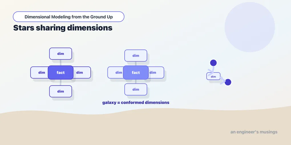
You’ve built a star: one fact table in the middle, denormalized dimensions on the points, single-key joins. It’s a good shape, and it has two well-known relatives that people reach for — one of them usually by mistake. Knowing all three isn’t trivia. It’s how you recognize when someone’s about to normalize your warehouse into a swamp, and how you spot the design decision that actually earns its keep. The whole chapter builds to one query — “units sold vs. units on hand, by title, by week” — and to the difference between the version that lies and the version that doesn’t.
The snowflake schema, and why it’s usually the wrong default
Look at dim_book. It repeats a genre string on every book — “Science Fiction” written out thousands of times, and next to it the category “Fiction” repeated even more. To a mind trained on transactional databases, that redundancy itches. The fix looks obvious: pull genre into its own dim_genre table, pull category into dim_category, and have each point at the next.
fct_order_items --- dim_book --- dim_genre --- dim_categoryThat’s a snowflake schema — dimensions normalized into sub-dimensions, so the star’s clean points fray into chains. You’ve traded some duplicated strings for referential tidiness. And on a columnar warehouse like Snowflake, that trade is almost always a loss.
The cost shows up the moment you write a query. In a flat star, “revenue by category” is a fact, one dimension, one join:
select
    b.category,
    sum(oi.quantity * oi.unit_price) as revenue
from fct_order_items as oi
join dim_book as b on oi.book_sk = b.book_sk
group by 1
Snowflake the schema and the same question grows a chain of joins, because category no longer lives on the book — it lives two hops away:
select
    c.category,
    sum(oi.quantity * oi.unit_price) as revenue
from fct_order_items as oi
join dim_book     as b on oi.book_sk    = b.book_sk
join dim_genre    as g on b.genre_sk    = g.genre_sk
join dim_category as c on g.category_sk = c.category_sk
group by 1
Every analyst now has to know that category isn’t on dim_book, that it hangs off dim_genre, that dim_genre in turn hangs off dim_category. The join graph is no longer “fact in the middle, dimensions on the points” — it’s a topology you have to memorize. Multiply that by every report, every ad-hoc question, every BI tool that has to be told about the extra tables, and you’ve made the warehouse harder to use in exchange for a saving that, on Snowflake, barely exists.
Here’s why the itch is misleading. The redundancy costs you almost nothing: Snowflake stores columns compressed, and a genre string that repeats ten thousand times compresses to nearly the footprint of storing it once. Dictionary and run-length encoding are exactly the case where a low-cardinality column repeated a million times collapses to a handful of distinct values plus pointers. So the “savings” you’re buying with normalization is largely imaginary — you’re normalizing to avoid a storage cost the storage engine already erased. What you’re paying is real: every query that filters or groups by category now threads two extra joins, every analyst has to know the chain exists, and the query planner has more tables to wrestle and more join orders to get wrong. You spent simplicity, the one currency the star was designed to hoard, to save disk that was already free.
When a snowflake is actually right
Don’t be dogmatic, though — the shape isn’t forbidden, it’s just rarely justified. There are two honest cases where snowflaking a sub-dimension out of the star earns its complexity.
A very large, very sparse sub-dimension. Suppose dim_book grew a rich cluster of attributes that only apply to a tiny fraction of titles — a detailed rights-and-licensing block that exists for the few hundred books the shop publishes itself, and is null for the hundreds of thousands it merely resells. Folding all of that into dim_book widens every row of a large table to carry columns almost none of them use. Splitting the licensing attributes into a dim_licensing sub-dimension that only the publisher-owned titles point at keeps the main dimension narrow and lets the sparse block stay small. The test is genuine sparsity plus genuine size: a wide attribute set that’s null for the overwhelming majority. Below that bar, keep it flat.
A security or governance boundary. Sometimes a group of attributes has to live in its own object because access to it is controlled separately — a sub-dimension holding regulated or restricted fields that only some roles may read, governed by its own masking policies and grants. Snowflaking it out isn’t about storage at all; it’s about drawing a permission boundary that a single wide dimension can’t express cleanly. If the reason you’re splitting is “these columns answer to a different owner or a different policy,” that’s a real reason, and it has nothing to do with duplicated strings.
Notice what’s not on the list: “to save space.” On a columnar warehouse that argument is mostly imaginary, and it’s the one people reach for most. Normalize for sparsity or for governance; never for the disk bill. Outside those cases, keep the star flat and let the storage be slightly larger. Simplicity wins the day-to-day, and the day-to-day is most days.
The galaxy: a constellation of facts
Now the shape that isn’t a mistake. Real warehouses have more than one business process to measure, and each gets its own fact table at its own grain. The bookshop measures sales in fct_order_items — one row per order line, additive measures like quantity and unit_price — and it measures inventory in fct_inventory_daily, a periodic snapshot with one row per book per day carrying that day’s stock_level. Two processes, two rhythms, two stars. When multiple fact tables share dimensions, you have a galaxy — also called a fact constellation, or a fact family.
        dim_date        dim_book
          |    \        /    |
          |     \      /     |
   fct_order_items    fct_inventory_daily
          |
     dim_customer
fct_order_items sits on dim_date, dim_book, and dim_customer. fct_inventory_daily sits on dim_date and dim_book only — inventory has no customer (nobody buys a snapshot). But the two dimensions in the middle, dim_date and dim_book, are shared. That sharing is the entire subject of the rest of this chapter. Get it right and the two stars combine into one integrated model you can query across. Get it wrong and you have two schemas that happen to live in the same database and can’t be compared — which is the most expensive kind of “almost.”
The word “share” is doing enormous work in that paragraph, and it’s worth being precise about what it has to mean.
Conformed dimensions: the actual point
A dimension is conformed when it’s used identically across multiple facts — the same table, the same keys, the same attributes, the same meaning. Not “a date dimension in each schema.” The date dimension, one model, referenced by both. When dim_date and dim_book are conformed between sales and inventory, something powerful falls out: you can slice both processes by the same calendar and the same book catalog and trust the comparison. “Units sold vs. units on hand, by title, by week” becomes a coherent question, and it’s only coherent because both facts are speaking the exact same dimensional language — the same book_sk means the same book on both sides, the same date_sk lands on the same calendar day.
Break conformance and the query silently lies. Let inventory quietly build its own book table with a different genre spelling, or a fiscal calendar that starts weeks on Monday while sales starts on Sunday, and “by title, by week” now compares two things that aren’t the same title and aren’t the same week — but the SQL runs, returns numbers, and nobody sees the seam. Conformed dimensions are the entire reason an integrated warehouse is more than a pile of disconnected reports. They’re what let a CFO drill from revenue to inventory to returns and land on the same rows every time. And they are only worth anything if you actually use them the right way — which brings us to the query this whole chapter has been circling.
Drill-across: the payoff, and the trap that ruins it
Two conformed dimensions across two facts unlock drill-across: pulling a measure from each fact and lining them up on the shared dimensions. “Units sold vs. units on hand, by title, by week” is the canonical drill-across — one measure (quantity) from fct_order_items, one measure (stock_level) from fct_inventory_daily, reported side by side against the same dim_book and the same weekly calendar off dim_date.
It is also the single easiest query in dimensional modeling to get catastrophically wrong. Here’s the wrong version — the one that looks reasonable and double-counts everything:
-- WRONG: one join across two facts fans out and inflates both measures
select
    b.title,
    d.week_start_date,
    sum(oi.quantity)     as units_sold,
    sum(inv.stock_level) as units_on_hand
from fct_order_items     as oi
join fct_inventory_daily as inv on inv.book_sk = oi.book_sk
join dim_book            as b   on b.book_sk   = oi.book_sk
join dim_date            as d   on d.date_sk   = oi.date_sk
group by 1, 2
Think about what the join produces before the group by ever runs. fct_order_items has many order lines per book, and fct_inventory_daily has one snapshot per book per day — so joining the two facts on book_sk pairs every order line for a title against every daily inventory row for that title, across all of time. A book with 300 order lines and a year of daily snapshots produces 300 × 365 rows for that one title. Now sum(oi.quantity) counts every order line 365 times, and sum(inv.stock_level) counts every snapshot 300 times. Both measures are inflated by the other fact’s row count. The numbers aren’t a little off — they’re off by two independent multipliers, and the multipliers change per title, so you can’t even eyeball the error. This is the classic fan-out (or chasm trap): the moment two many-rows facts meet in a single join, their measures multiply.
Tightening the join doesn’t save you. Add and inv.date_sk = oi.date_sk so the facts only meet on the same day and the explosion shrinks — but it doesn’t vanish. A title with three order lines on a day that also has one inventory snapshot still yields three rows, so stock_level is counted three times for that day. Any grain at which both facts have more than one row per group re-opens the trap. There is no join condition that fixes this, because the problem isn’t the condition — it’s that you asked one join to serve two facts at two grains.
The right shape is drill-across: aggregate each fact to the conformed grain separately, then join the two results on the conformed keys. Each fact is summarized on its own, to one row per book per week, so neither can inflate the other. Then — and only then — you line them up.
-- RIGHT: aggregate each fact to the conformed grain first, then join on the keys
with sales_by_week as (
    select
        oi.book_sk,
        d.iso_year,
        d.iso_week,
        sum(oi.quantity) as units_sold
    from fct_order_items as oi
    join dim_date as d on oi.date_sk = d.date_sk
    group by 1, 2, 3
),

on_hand_by_week as (
    -- stock_level is SEMI-ADDITIVE: it sums across books but NEVER across days.
    -- The week's on-hand is the last snapshot in the week, not the sum of seven.
    select book_sk, iso_year, iso_week, stock_level as units_on_hand
    from (
        select
            inv.book_sk,
            d.iso_year,
            d.iso_week,
            inv.stock_level,
            row_number() over (
                partition by inv.book_sk, d.iso_year, d.iso_week
                order by inv.snapshot_date desc
            ) as rn
        from fct_inventory_daily as inv
        join dim_date as d on inv.date_sk = d.date_sk
    )
    where rn = 1
)

select
    b.title,
    coalesce(s.iso_year, h.iso_year) as iso_year,
    coalesce(s.iso_week, h.iso_week) as iso_week,
    coalesce(s.units_sold,   0)      as units_sold,
    coalesce(h.units_on_hand, 0)     as units_on_hand
from sales_by_week as s
full outer join on_hand_by_week as h
       on  s.book_sk  = h.book_sk
       and s.iso_year = h.iso_year
       and s.iso_week = h.iso_week
join dim_book as b on b.book_sk = coalesce(s.book_sk, h.book_sk)
order by b.title, iso_year, iso_week
Three things in that query are the whole lesson. First, each measure is summed inside its own CTE, at the same (book_sk, iso_year, iso_week) grain, so no fact ever multiplies another — units_sold and units_on_hand are each computed exactly once. Second, the two aggregates meet through a full outer join on the conformed keys, not an inner join: a title that sold in a week but had no inventory snapshot (or a title held in stock that sold nothing) still appears, with a zero on the missing side instead of vanishing. An inner join here would quietly drop exactly the rows an analyst most wants to see — the stockout that sold nothing, the fire-sale that emptied the shelf. Third, notice the comment on on_hand_by_week: inventory’s stock_level is semi-additive, so you never sum it across days. Summing a week of daily snapshots would answer “how much stock-day did we hold,” which is not a number anyone asked for. The week’s on-hand is a point-in-time value — here, the last snapshot in the week via row_number(). Averaging the seven days is the other defensible choice; summing them is always wrong.
That’s drill-across: separate aggregations, each grouped to the conformed grain, joined on the conformed keys. It’s more SQL than the fan-out version, and every extra line is there to stop a specific way the one-join version lies.
Shrunken dimensions and aggregate rollups
The drill-across above computed the week grain on the fly by grouping on iso_year and iso_week off dim_date. If you do that in ten reports, you’ve re-derived “week” ten times, and the tenth analyst will group on week_start_date instead of iso_week and get subtly different buckets. The fix is a shrunken dimension (also called a rollup dimension): a conformed dimension at a coarser grain, whose attributes are a strict, agreeing subset of the base dimension’s. A week dimension shrunk down from dim_date:
-- models/marts/dim_week.sql  — a shrunken rollup of the conformed dim_date
select
    {{ dbt_utils.generate_surrogate_key(['iso_year', 'iso_week']) }} as week_sk,
    iso_year,
    iso_week,
    min(date_day) as week_start_date,
    max(date_day) as week_end_date
from {{ ref('dim_date') }}
group by iso_year, iso_week
dim_week is conformed by construction — it’s built from dim_date, so its weeks can’t disagree with the daily calendar they’re aggregated from. Its week_sk follows the same surrogate-key discipline as every other dimension (generate_surrogate_key, natural attributes iso_year/iso_week inside). And it pairs with an aggregate fact — agg_sales_weekly at (book_sk, week_sk) grain — so the common “units by week” question hits a small pre-summarized table conformed to dim_book and dim_week, instead of scanning atomic order lines every time. The rule that keeps a shrunken dimension honest: its attributes must roll up cleanly from the base. iso_week and week_start_date do; day_name doesn’t (a week has seven), so it simply doesn’t appear on dim_week. A shrunken dimension is a subset that agrees, never a summary that improvises. (Aggregate navigation — routing a query to the coarsest table that can answer it — is its own topic, and the aggregates and semantic-layer chapter picks it up.)
The bus matrix as a planning deliverable
Conformance across two facts is easy to hold in your head. Across twenty, it’s a design you have to plan, and the planning artifact is the bus matrix: business processes down the rows, conformed dimensions across the columns, an X where a process uses a dimension. It’s the whole data-warehouse plan on one page — what you’ll build, and which dimensions must conform across all of it. For the bookshop it’s small enough to read at a glance:
                    | dim_date | dim_book | dim_customer
--------------------|----------|----------|-------------
Sales (order items) |    X     |    X     |      X
Inventory (daily)   |    X     |    X     |
Returns             |    X     |    X     |      X
The matrix is a planning deliverable, not documentation you write afterward — it’s meant to exist before the second fact table does. Read a column and you see every process that must agree on that dimension: dim_date and dim_book are used by all three processes, which is precisely why they’re the ones that have to conform, and why a drift in either breaks the most queries. Read a row and you see one star’s dimensions — one fact table’s worth of design. Read it top to bottom and you’ve scoped the warehouse: three facts, three conformed dimensions, a build order. Plan the matrix first and conformance is designed in — every new fact snaps onto dimensions that already agree. Discover it later and you’re retrofitting agreement onto tables that already disagree, which is the year-long reconciliation project nobody budgets for.
Conformance is a ref() you already wrote
The reassuring part: in dbt, conformed dimensions aren’t extra work — they’re what you get for free, provided you mint keys the way the dimensions chapter argued for. Look again at how fct_inventory_daily was built back in chapter 05:
-- models/marts/fct_inventory_daily.sql
select
    {{ dbt_utils.generate_surrogate_key(['book_id', 'snapshot_date']) }} as inventory_sk,

    {{ dbt_utils.generate_surrogate_key(['book_id']) }}       as book_sk,
    {{ dbt_utils.generate_surrogate_key(['snapshot_date']) }} as date_sk,

    snapshot_date,
    stock_level
from {{ ref('stg_inventory') }}
Notice what is not there: any join to dim_book or dim_date. And yet the book_sk this fact carries is byte-identical to the one fct_order_items carries, and both resolve into the same dim_book row. That’s the payoff of a deterministic surrogate key. Because dim_book mints its key as generate_surrogate_key(['book_id']) and every fact mints its foreign key with the same expression over the same natural key, the two agree by construction. Conformance is arithmetic, not a lookup.
This is precisely why the dimensions chapter argued against sequence-generated keys. Had dim_book.book_sk been a row_number() or an identity column, neither fact could compute it — each would have to join to the dimension to look its key up, on every build, forever. That works, and plenty of warehouses do it, but it makes every fact build depend on the dimension being present and current, and it makes a rebuilt dimension silently renumber keys that facts have already stored. Hashing the natural key removes the join and the hazard together.
So there’s no “inventory calendar” that can drift from the “sales calendar,” because there is only one calendar and both facts arrive at its keys independently and identically. Conformance isn’t a feature you switch on; it’s what happens when two facts derive their keys from the same natural keys with the same expression, and you resist the urge to copy the dimension. dbt’s DAG makes the shared node the path of least resistance — the lazy choice and the correct choice are the same choice.
Proving it: one relationships test, two facts
“Both facts point at the same dimension” is a claim, and claims in a warehouse should be executable. dbt’s relationships test makes it one — it fails the build if any fact key points at a dimension row that doesn’t exist. Point both facts’ keys at the same ref('dim_date') and ref('dim_book'), and the test doesn’t just check referential integrity — it encodes conformance as an assertion:
# models/marts/_marts.yml
models:
  - name: fct_order_items
    columns:
      - name: date_sk
        data_tests:
          - relationships: {to: ref('dim_date'), field: date_sk}
      - name: book_sk
        data_tests:
          - relationships: {to: ref('dim_book'), field: book_sk}

  - name: fct_inventory_daily
    columns:
      - name: date_sk
        data_tests:
          - relationships: {to: ref('dim_date'), field: date_sk}
      - name: book_sk
        data_tests:
          - relationships: {to: ref('dim_book'), field: book_sk}
Four tests, and the load-bearing detail is that all four to: clauses name the same two models. fct_order_items.date_sk and fct_inventory_daily.date_sk both have to resolve into dim_date — the one, conformed dim_date. If someone ever forks a second calendar for inventory, this YAML still points inventory’s date_sk at the original dim_date, so the moment the fork’s keys stop matching, the test goes red on dbt build. The bus matrix said dim_date and dim_book must conform across every process; these tests are that row-and-column agreement turned into a tripwire. Since Snowflake accepts FOREIGN KEY constraints but doesn’t enforce them, this test is the only referee that both stars are still sharing the same sky — and it runs on every build, forever.
Final thoughts
The snowflake schema is the shape to argue against — it optimizes for a scarcity, storage, that columnar warehouses eliminated, and charges you complexity for the privilege; keep it in your pocket for genuinely sparse sub-dimensions and governance boundaries, and nothing else. The galaxy is the shape you’ll actually grow into, and conformed dimensions are the reason it holds together instead of fragmenting into a dozen reports that can’t be compared. But conformance only pays off if you drill across correctly: aggregate each fact to the conformed grain on its own, then join on the shared keys — never one fan-out join that multiplies both measures into fiction. Get the bus matrix right and every new fact table snaps onto dimensions that already agree; back it with a relationships test per key and the agreement stops being a promise and becomes a build step. The shape of one star barely matters. Whether your stars share their sky — and whether you query across it without double-counting — is the whole game.
Comments