Three Kinds of Fact Table (and the Factless One)

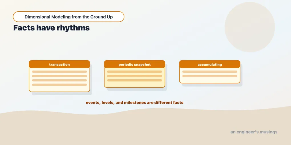
fct_order_items answers a lot of questions, but not all of them. It can tell you how many copies of a title sold last Tuesday. It cannot tell you how many copies were in stock last Tuesday, or how long the average order takes to travel from placed to delivered. Those aren’t harder queries against the same fact — they’re different kinds of fact table, because they measure the business at a different rhythm.

Kimball names three, and then a fourth that has no measures at all. The rhythm is the whole distinction, and by the end of this chapter you’ll have built one of each — including the accumulating snapshot, fct_orders, that later chapters keep coming back to.

Transaction facts: one row per event

You already built one. A transaction fact records an atomic event the instant it happens — one row per order line, born when the line is created and never touched again. The grain is an event, the measures are additive, and the table only grows. This is the workhorse — most facts you build are transaction facts, and it’s the right default when you’re unsure which type you need.

Its blind spot is anything that’s true between events. Inventory doesn’t get “transacted” on a quiet day — the stock level just persists. A pure event log can’t tell you the state of the world on a day when nothing happened, and “how many were in stock on the 14th” is exactly that question. You could, in principle, replay every stock movement since the beginning of time and reconstruct the level — and that’s precisely the query you don’t want every dashboard running at 9 a.m. When the reconstruction is the point, you want a different table.

Periodic snapshots: one row per entity per period

A periodic snapshot takes a photograph on a fixed cadence — one row per entity per period, whether or not anything changed. A daily inventory fact holds one row per book per day, carrying that day’s stock level. Monday: 40. Tuesday: 40. Wednesday: 37. Three rows, one per day, even though nothing moved on Tuesday.

The measures here are usually semi-additive — that inventory level sums across books but never across days, exactly as the last chapter warned. Snapshots trade storage for the ability to answer state-of-the-world questions directly, and for anything you snapshot daily, that’s a trade worth making. The storage math is honest, though: a thousand titles snapshotted daily is 365,000 rows a year — trivial. A hundred million SKUs snapshotted daily is not, and at that scale you start snapshotting weekly, or only what moved plus a periodic full baseline. For the bookshop, daily and complete is the right answer.

The photograph nobody takes for you

Here’s the part most write-ups skip: the source system almost never hands you one clean row per book per day. Real sources come in two shapes, and each needs its own build.

Shape one: the source only knows now. The operational database has a stock_level column holding the current value, full stop. The only way to get history is to start photographing — each dbt run appends today’s state, and history accumulates from the day you begin. That’s the easy build (we’ll do it below), with one hard limitation you should say out loud to stakeholders: you cannot backfill a photograph you never took. Miss a day’s run and that day is a hole forever. History starts when the snapshot starts, not when the business did.

Shape two: the source gives you a movement stream. Every receipt, sale, and adjustment lands as a delta — book_id, timestamp, +40 or -3. Now the level is derivable for any day, including days before the warehouse existed, but somebody has to derive it. That somebody is a window function.

From movements to end-of-day levels

The derivation has two steps: net the movements per book per day, then turn deltas into levels with a running sum. There’s a trap in the middle — a running sum over only the days that have movements skips the quiet days, and a snapshot with missing days isn’t a snapshot. So you build a spine of every day, cross-join it with every book, and let the quiet days contribute zero:

-- models/intermediate/int_inventory_eod.sql
{{ config(materialized='table') }}

with movements as (
    select * from {{ ref('stg_inventory_movements') }}
),

daily_net as (
    select
        book_id,
        cast(moved_at as date)  as movement_date,
        sum(quantity_delta)     as net_change
    from movements
    group by book_id, cast(moved_at as date)
),

spine as (
    {{ dbt_utils.date_spine(
        datepart="day",
        start_date="to_date('2024-01-01')",
        end_date="dateadd(day, 1, current_date)"
    ) }}
),

books as (
    select distinct book_id from daily_net
),

book_days as (
    select b.book_id, s.date_day
    from books b
    cross join spine s
),

levels as (
    select
        bd.book_id,
        bd.date_day as snapshot_date,
        sum(coalesce(dn.net_change, 0)) over (
            partition by bd.book_id
            order by bd.date_day
            rows between unbounded preceding and current row
        ) as stock_level
    from book_days bd
    left join daily_net dn
      on  dn.book_id      = bd.book_id
      and dn.movement_date = bd.date_day
)

select * from levels

The cross join manufactures the full grain — every book on every day — and the left join hangs that day’s net change on it, or nothing. The cumulative sum(coalesce(net_change, 0)) then does two jobs at once: it turns deltas into a level, and it carries the level forward across quiet days, because adding zero is carrying forward. Tuesday’s row exists and says 40, even though Tuesday said nothing.

Two footnotes on this build. First, it assumes the movement stream is complete from a zero starting point — if the shop opened with stock on the shelf, seed an opening-balance movement per book, or every level is off by the opening amount forever. Second, some sources post sparse levels rather than deltas — a new stock_level only on days it changes. The carry-forward for that shape is last_value with ignore nulls:

last_value(sparse_level) ignore nulls over (
    partition by book_id
    order by date_day
    rows between unbounded preceding and current row
) as stock_level

Same spine, same cross join — only the gap-filling function changes.

The snapshot fact itself

However the end-of-day level got made — photographed from current state (shape one) or derived from movements (shape two, in which case stg_inventory is a thin view over int_inventory_eod) — the fact build is the same. One row per book per day, appended incrementally:

-- models/marts/fct_inventory_daily.sql
{{
    config(
        materialized='incremental',
        unique_key='inventory_sk',
        incremental_strategy='merge'
    )
}}

with inventory as (
    select * from {{ ref('stg_inventory') }}
)

select
    {{ dbt_utils.generate_surrogate_key(['book_id', 'snapshot_date']) }} as inventory_sk,

    {{ dbt_utils.generate_surrogate_key(["coalesce(book_id, '-1')"]) }}       as book_sk,
    {{ dbt_utils.generate_surrogate_key(['snapshot_date']) }} as date_sk,

    snapshot_date,
    stock_level        -- semi-additive: sums across books, never days

from inventory

{% if is_incremental() %}
where snapshot_date > (select max(snapshot_date) from {{ this }})
{% endif %}

The grain is stamped into the primary key — book_id + snapshot_date, hashed — and the dimension keys use the same generate_surrogate_key expressions as everywhere else, so book_sk joins straight to dim_book and date_sk to dim_date. The merge on inventory_sk means re-running a day corrects that day’s photograph in place instead of doubling it.

Proving the semi-additive rule

“Never sum a level over time” is easy to nod along to and easy to violate at 5 p.m. on a Friday, so let’s watch it lie. Say Gardening for Introverts held 40, 40, and 37 copies across Monday through Wednesday. The query someone will inevitably write:

-- WRONG: sums a level across days
select b.title, sum(f.stock_level) as stock
from fct_inventory_daily f
join dim_book b on b.book_sk = f.book_sk
where f.snapshot_date between '2026-05-11' and '2026-05-13'
group by b.title;

That returns 117 — a number with units of copy-days that will be read as “117 copies in stock,” triple the truth, formatted with the same confidence as a correct one. The dimensions of the mistake matter: the more days in the filter, the bigger the lie, so a quarter-to-date dashboard inflates by ninety-ish and nobody can say why the numbers “drift up.”

The honest queries pick a stance on time instead of summing across it:

-- state on one chosen day: filter time to a point, then sum across books
select sum(stock_level) as copies_in_shop
from fct_inventory_daily
where snapshot_date = '2026-05-13';

-- period-end: the level on the last day of each month
select b.title, f.stock_level as month_end_stock
from fct_inventory_daily f
join dim_book b on b.book_sk = f.book_sk
qualify row_number() over (
    partition by f.book_sk, date_trunc('month', f.snapshot_date)
    order by f.snapshot_date desc
) = 1;

-- average daily level across the period: honest, and says so in its name
select b.title, avg(f.stock_level) as avg_daily_stock
from fct_inventory_daily f
join dim_book b on b.book_sk = f.book_sk
where f.snapshot_date between '2026-05-01' and '2026-05-31'
group by b.title;

Pin time to a point, take the period-end value, or average over the period — those are the three legal moves with a semi-additive measure. Snowflake’s qualify makes the period-end one a single readable query instead of a subquery sandwich.

Accumulating snapshots: one row per process, updated as it moves

An accumulating snapshot breaks the append-only rule on purpose. It models a process with a known set of milestones, keeps one row per instance of that process, and updates that row as the instance advances through the milestones.

An order’s fulfillment is the textbook case. One row per order, with a foreign key to the date dimension for each milestone — ordered, shipped, delivered — most of them unfilled at first. The order is placed, so the order date is set; it ships, it arrives, and each event updates the same row in place. Alongside the dates sit lag measures — days from order to ship, days from ship to delivery — that only become computable as the later dates land.

This is the fact that answers “how long does fulfillment take, and where do orders stall?” A transaction fact can’t: the milestones are separate events scattered across separate rows, and stitching them back into a per-order timeline is the join marathon the star was supposed to kill. The accumulating snapshot does the stitching once, at build time.

Building fct_orders

This table matters beyond this chapter — the role-playing-dimension work and the testing chapter both build directly on it — so let’s pin down its contract before writing a line of SQL. Grain: one row per order_id. Columns: the degenerate order_id, a customer_sk, three milestone date keys (order_date_sk, ship_date_sk, delivery_date_sk), the current order_status, and two lag measures (days_to_ship, days_to_deliver).

The source is stg_orders, which carries the milestone columns the operational system updates in place — order_date, ship_date, delivery_date, order_status — with the later dates null until they happen. (If your source instead emits milestone events — a shipped row, a delivered row — pivot them to columns first with a conditional aggregation: min(case when event_type = 'shipped' then event_date end) per order, grouped by order_id. Same destination, one extra staging hop.)

-- models/marts/fct_orders.sql
{{
    config(
        materialized='incremental',
        unique_key='order_id',
        incremental_strategy='merge'
    )
}}

with orders as (
    select * from {{ ref('stg_orders') }}
)

select
    order_id,                                                    -- degenerate dimension & merge key

    {{ dbt_utils.generate_surrogate_key(["coalesce(customer_id, '-1')"]) }}     as customer_sk,
    {{ dbt_utils.generate_surrogate_key(['order_date']) }}      as order_date_sk,
    {{ dbt_utils.generate_surrogate_key(['ship_date']) }}       as ship_date_sk,
    {{ dbt_utils.generate_surrogate_key(['delivery_date']) }}   as delivery_date_sk,

    order_status,

    datediff('day', order_date, ship_date)                      as days_to_ship,
    datediff('day', ship_date,  delivery_date)                  as days_to_deliver

from orders

{% if is_incremental() %}
where order_id in (
        select order_id from {{ this }}
        where order_status not in ('delivered', 'cancelled')
      )
   or order_id not in (select order_id from {{ this }})
{% endif %}

Walk the mechanics, because every line is doing accumulating-snapshot work.

The merge key is the grain. unique_key='order_id' with the merge strategy is what makes this an accumulating snapshot at all: when a re-selected order comes through, Snowflake’s MERGE matches it by order_id and updates the existing row — the milestone columns fill in, in place, exactly as the pattern demands. A transaction fact merges to correct mistakes; this table merges as its normal mode of life.

The incremental filter selects “everything still in motion.” On each run we reprocess two sets: orders the fact already has whose status isn’t terminal — they may have advanced since we last looked — and orders the fact has never seen. An order sits in the reprocess set from placement until it hits delivered or cancelled, getting re-merged on every run; the moment it goes terminal it stops being selected and its row goes quiet forever. (The not in subqueries are safe here precisely because order_id is the merge key — it can never be null in {{ this }}, which is the one condition under which not in betrays you.) If fulfillment can take months, this stays cheap: the working set is only the open orders, not history.

Unfilled milestones still get a key. Look at what generate_surrogate_key(['ship_date']) does when ship_date is null: the macro coalesces the null to a sentinel string before hashing, so an unshipped order gets a real, deterministic, not-null ship_date_sk — the same hash for every pending milestone everywhere in the warehouse. Right now that key points at nothing; the next chapter builds the unknown-member row in every dimension that it will land on, and chapter 7 gives dim_date its “hasn’t happened yet” row. The discipline — fact foreign keys are never null — starts here, even before the row it depends on exists.

The lag measures land when the milestones do. datediff returns null while either endpoint is null, so days_to_ship is null until the order ships, then becomes a plain additive-enough number you can average and percentile. Watch one order move through three runs:

run	order_status	ship_date_sk	delivery_date_sk	days_to_ship	days_to_deliver
Day 1	placed	(pending hash)	(pending hash)	null	null
Day 4	shipped	✓ real date key	(pending hash)	3	null
Day 9	delivered	✓	✓ real date key	3	5

Same row, three states — the table is a scoreboard, not a ledger. avg(days_to_ship) across delivered orders is your fulfillment SLA; count(*) of rows stuck in shipped for more than a week is your stall report. Both are one-liners now.

Two design notes before you copy this pattern

Milestone dates are roles, not tables. order_date_sk, ship_date_sk, and delivery_date_sk all point at the same dim_date — one calendar playing three parts. That’s a role-playing dimension, and chapter 13 covers how to query it without the three joins tripping over each other. What you don’t do is build three date dimensions.

Decide which version of the customer this row means. fct_orders has one row per order but the customer it points at can change — and once dim_customer becomes slowly changing (chapter 8), “the customer” is really “a version of the customer.” Kimball’s convention for accumulating snapshots is to freeze the dimension keys at the version in effect when the process began, and that’s the sane default: the order was placed by the Boston version of customer 2, and re-pointing it to Denver later would quietly rewrite regional history. Our hash-of-natural-key customer_sk sidesteps the question for now; when versioned keys arrive in chapter 8, remember this paragraph.

Factless facts: the event with no number

Sometimes the thing worth recording has no number attached, and a factless fact — a row of nothing but foreign keys — records it anyway. There are two distinct flavors, and they answer opposite questions.

Event factless facts record that something happened. A customer adds a book to their wishlist: that’s a real business event with real analytical value — which titles generate desire, which desires convert to sales — and no measure in sight. The fact is three keys and nothing else:

-- models/marts/fct_wishlist_adds.sql
{{ config(materialized='table') }}

select
    {{ dbt_utils.generate_surrogate_key(["coalesce(customer_id, '-1')"]) }} as customer_sk,
    {{ dbt_utils.generate_surrogate_key(["coalesce(book_id, '-1')"]) }}     as book_sk,
    {{ dbt_utils.generate_surrogate_key(['added_date']) }}  as date_sk

from {{ ref('stg_wishlists') }}

The measure, when you need one, is count(*) — wishlist adds per title per week is a group-by away. Some modelers add a literal 1 as wishlist_add_count column so BI tools have something to drag into the measures well; it’s harmless and slightly silly, and either choice is fine.

Coverage factless facts record that something was eligible — a condition that held, rather than an event that fired. The bookshop runs a summer promotion covering some titles: which books did it cover? Coverage isn’t a quantity and it isn’t an event with a timestamp — it’s a state of the world you need to slice by:

-- models/marts/fct_promotion_coverage.sql
{{ config(materialized='table') }}

select
    {{ dbt_utils.generate_surrogate_key(['pb.promotion_id']) }} as promotion_sk,
    {{ dbt_utils.generate_surrogate_key(['pb.book_id']) }}      as book_sk

from {{ ref('stg_promotion_books') }} pb

The grain is one row per promotion per covered book, and dim_promotion — a small dimension off stg_promotions with the name and the date range — gives the rows their words.

Counting the absence

Here’s why the coverage table earns its keep. “Which promoted titles sold?” needs no factless fact — the sales are in fct_order_items. But “which promoted titles didn’t sell?” is a question about rows that don’t exist, and you cannot query rows that don’t exist unless some table asserts what should have been possible. Coverage is that assertion, and the query is an anti-join between what was covered and what sold:

with covered as (
    select c.book_sk
    from fct_promotion_coverage c
    join dim_promotion p on p.promotion_sk = c.promotion_sk
    where p.promotion_name = 'Summer Reading 2026'
),

sold as (
    select distinct oi.book_sk
    from fct_order_items oi
    join dim_date d on d.date_sk = oi.date_sk
    where d.date_day between '2026-06-01' and '2026-08-31'
)

select b.title, b.author
from covered c
join dim_book b on b.book_sk = c.book_sk
left join sold s on s.book_sk = c.book_sk
where s.book_sk is null
order by b.title;

The left join … where … is null is the anti-join: every covered book, minus the ones with at least one sale in the window, equals the promotion’s dead weight. The same shape answers “which enrolled students missed class” and “which insured properties never claimed” — any time the business asks about an absence, look for the coverage fact that makes the absence computable.

Timespan facts, briefly

One more rhythm deserves a name before we move on. A timespan fact carries a state and the window it held for — one row per book per price regime, say, with valid_from, valid_to, and the list_price that ruled between them. It’s the answer when the question is “what was the price when this order happened” and the source only keeps the current price.

If that structure sounds familiar, it should: it’s the same effective-dated windowing that slowly changing dimensions use, and chapter 8 treats it properly. The line between a timespan fact and a Type 2 dimension is what the windowed thing is — a measure you’ll aggregate belongs in a fact with a window; descriptive context you’ll slice by belongs in a dimension with a window. Same machinery, different seat at the table.

Testing the grain, per type

Every fact type declares a grain, and every grain deserves a test that fails the day someone’s join quietly fans it out. The test differs by type because the grain does:

# models/marts/_facts.yml
models:
  - name: fct_order_items          # transaction: one row per order line
    columns:
      - name: order_item_sk
        data_tests: [unique, not_null]

  - name: fct_inventory_daily      # periodic snapshot: one row per book per day
    data_tests:
      - dbt_utils.unique_combination_of_columns:
          combination_of_columns:
            - book_sk
            - snapshot_date
    columns:
      - name: inventory_sk
        data_tests: [unique, not_null]

  - name: fct_orders               # accumulating snapshot: one row per order
    columns:
      - name: order_id
        data_tests: [unique, not_null]

  - name: fct_promotion_coverage   # coverage factless: one row per promotion-book
    data_tests:
      - dbt_utils.unique_combination_of_columns:
          combination_of_columns:
            - promotion_sk
            - book_sk

The transaction fact and the accumulating snapshot each have a single-column grain, so plain unique does the job — and note that for fct_orders the grain test rides on the degenerate dimension, which is pleasingly literal: the grain is the order, so the order id is unique. The snapshot and the coverage fact have composite grains, and dbt_utils.unique_combination_of_columns states them outright — which doubles as documentation, since the test YAML now says “one row per book per day” in executable form. When the movement-stream build upstream double-counts a day, this is the test that catches it before a dashboard does.

You’ll want more than one

The instinct is to build the one true fact table for a business process. Resist it. Sales is a process, and it wants a transaction fact for what sold, a periodic snapshot for daily inventory levels, and an accumulating snapshot for fulfillment timing. Same process, three facts, three rhythms — each answering questions the others structurally can’t. Picking the type is picking the question you’re willing to answer fast.

Final thoughts

“What kind of fact table” isn’t a modeling technicality — it’s a decision about what the business is allowed to ask and how fast. Transaction facts capture flows, snapshots capture levels, accumulating snapshots capture progress, and factless facts capture that something merely happened — or was merely possible. Get the rhythm wrong and you’ll be reconstructing it in every query, forever, in SQL that gets copy-pasted until it’s wrong somewhere. Get it right and the hard questions become one-liners: the stall report is a count(*), the dead-promotion list is an anti-join, the month-end stock is a qualify. Most real processes need more than one of these, and that’s not redundancy — it’s the point.

Next: Dimension Tables and Surrogate Keys