Human Review: Trust as a Measurement Discipline

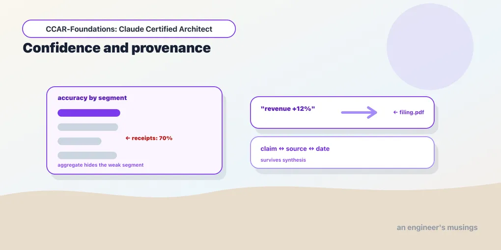
An extraction pipeline is 99% accurate on digital invoices and 70% accurate on handwritten receipts. If digital invoices dominate the traffic, its overall score looks reassuring while receipts still need close review. Decide where oversight can be reduced from those segment results, and retain the evidence needed to investigate an individual error.

Exam objectives covered here. 5.5 Design human review workflows and confidence calibration. 5.6 Preserve information provenance and handle uncertainty in multi-source synthesis. Numbering follows the Claude Certified Architect – Foundations Exam Guide, version 1.0, effective July 2026.

What review, confidence, and provenance are for

Removing human review is where the value is, and it is also where systems quietly break. The whole point of automating extraction or synthesis is to stop paying for a person to check every output, so there is real pressure to look at a headline accuracy number, decide it is good enough, and turn the reviewers off. The headline number is the thing most likely to be lying to you, and review measurements are how you find out which outputs still need attention. Provenance keeps each claim connected to the source that supports it, so a later reviewer can check the answer.

These are the Structured Extraction and Multi-Agent Research scenarios at their most rigorous. The measurement content of this chapter is standard statistics, worked out below with the numbers shown so you can check them. The mechanisms it reaches for are introspected from the installed packages rather than described from memory: the citation types, the permission callbacks, the judge’s forced tool call. Everything that needs a live model call is marked as such.

Why it matters, and the number that tempts you to skip it

A high overall accuracy figure can create pressure to stop reviewing outputs. Before doing so, inspect the segments that contribute to the average and the consequences of errors within each.

Reduce review where the evidence supports it, and keep measuring the outputs that now pass automatically. Allocate the remaining capacity to the segments and error types that need it.

The aggregate-accuracy trap

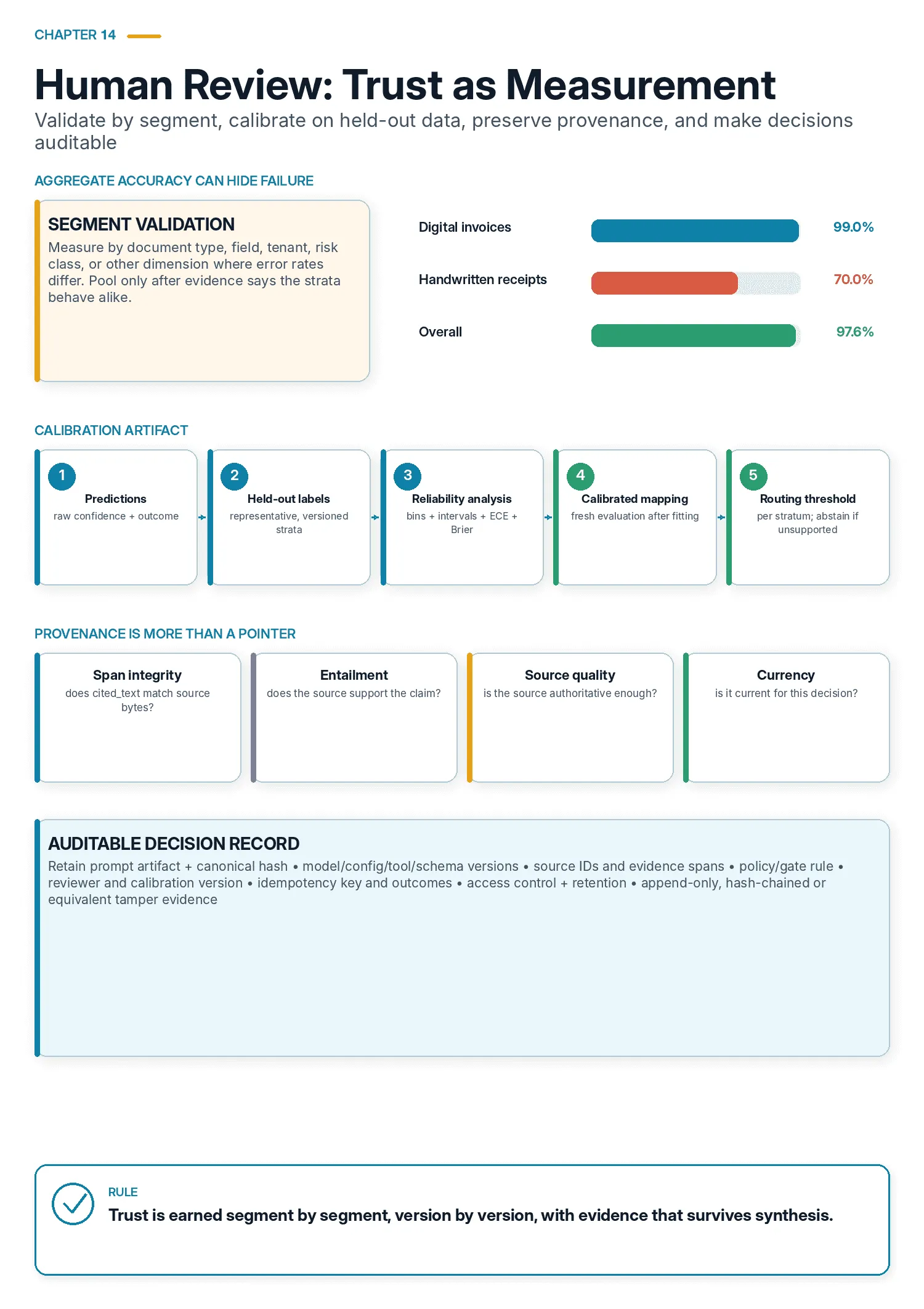
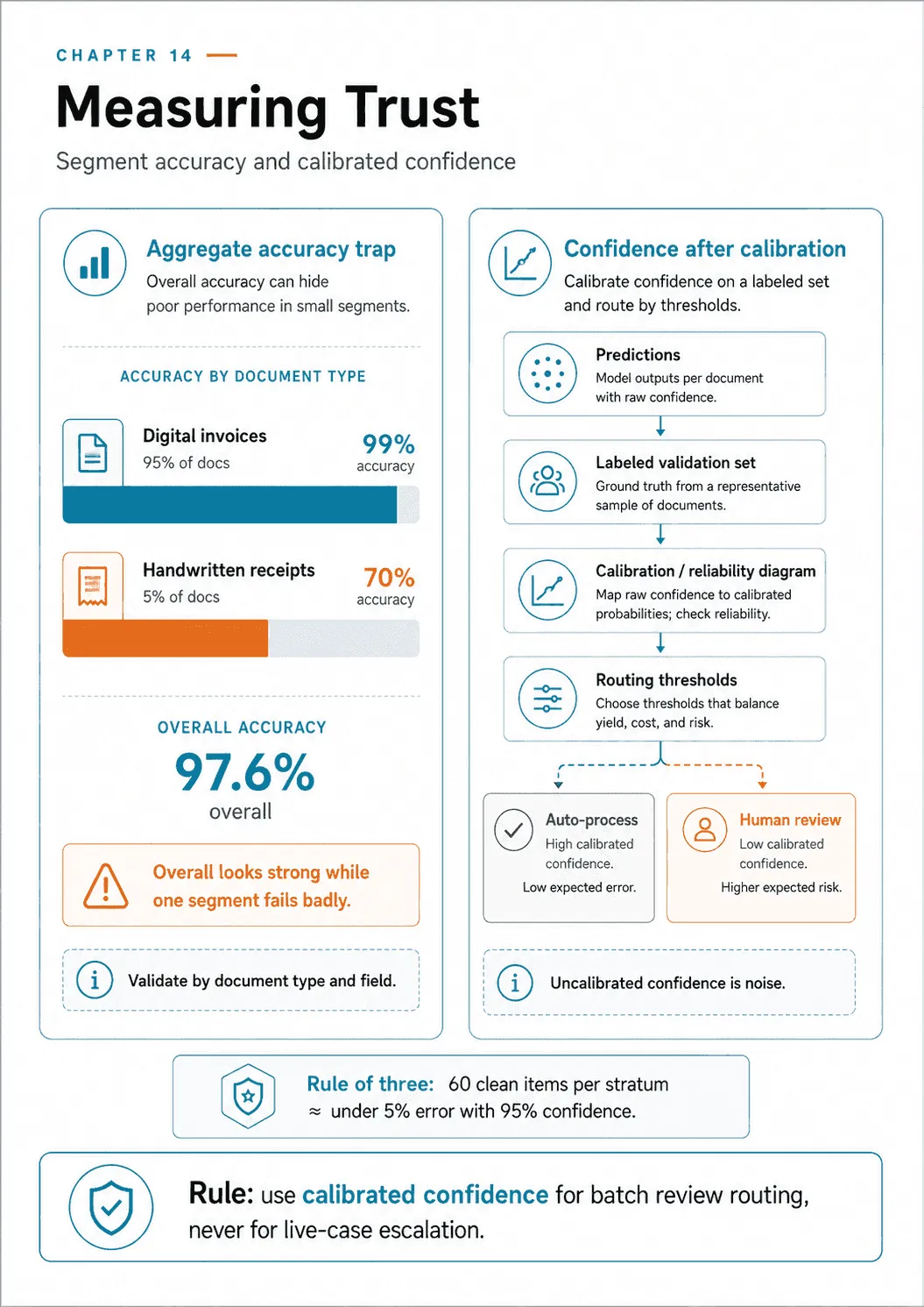
An aggregate accuracy number hides per-segment failure. “97% accurate overall” sounds like a system ready to automate. It can be masking 99% on invoices and 70% on handwritten receipts, or excellent on total and poor on tax_id; the average washes out the segments that are failing, and automating on the strength of it ships the failures. So measure by document type and field.

The arithmetic makes it concrete. Suppose 95% of your documents are clean digital invoices at 99% accuracy, and 5% are handwritten receipts at 70%. The blended figure is 0.95 x 0.99 + 0.05 x 0.70 = 0.9755, or 97.6% overall. That number is true. It is also compatible with three out of ten handwritten receipts being wrong, forever and silently. The failures land on exactly the documents a human would have flagged in two seconds. The aggregate did not lie — it averaged.

Set an acceptance threshold for each relevant segment and collect evidence against it before reducing review. The digital-invoice result cannot establish that handwritten receipts meet the same threshold.

How many samples, actually

There are two different questions, and they need different numbers.

Question one: is the error rate below my threshold? You want assurance, not a point estimate. The rule of three is the tool. Review n items and find zero errors, and you can be about 95% confident the true error rate is below 3/n. Invert it:

target error rate   n with zero errors observed
   5%                  3 / 0.05  =  60
   2%                  3 / 0.02  = 150
   1%                  3 / 0.01  = 300

Under the assumptions below, sixty error-free observations support an approximate 95% upper bound of 5% on that stratum’s error rate.

Before you spend it, know what you are buying. The rule of three is a shortcut with four load-bearing assumptions, and every one of them fails in a real pipeline in a recognizable way.

• The observations are independent. Errors have to be one-per-item, not clustered. They rarely are. One customer sends four hundred invoices on the same broken template, one OCR batch is skewed, one upstream vendor changes a form. Sixty items drawn from twenty documents is not sixty observations, and the interval you compute from it is narrower than the truth. If your errors arrive in clumps, sample and analyse at the level of the clump — the template, the vendor, the batch — not the row.
• The sample is representative of the population you are gating. Sampling last month’s traffic and automating next month’s is an assumption about drift, not a measurement. Sampling only what a reviewer already flagged measures the flagged population and nothing else. Draw at random from the exact stream the gate will run on.
• The observations are Bernoulli — each item is cleanly right or wrong under a rubric fixed before you look. If graders disagree about what counts as an error, or the rubric moves while you sample, you have not measured a rate. Fix the rubric first and check that two graders agree on it.
• Zero errors were observed. This is the one people quietly break, and it is the subject of the next two paragraphs.

The bound is also a bound on the stratum you sampled, and only that one. Sixty clean handwritten receipts say nothing about digital invoices, and sixty items drawn across both say something about a blend that will shift the moment your traffic mix does. That is the whole reason this chapter stratifies: the shortcut is cheap precisely because it is narrow.

Note the clause that makes it cheap: zero errors observed. The rule of three is a shortcut that only applies when nothing failed. Find one error in your sixty and you have not lost the ability to bound the rate — you have lost the shortcut. Inference still works; the arithmetic just gets less flattering, and you have to say which interval you mean:

1 error in 60, all at 95%
  exact (Clopper-Pearson), one-sided upper bound   7.66%    <- compare this to the 5%
  exact (Clopper-Pearson), two-sided interval      0.04% - 8.94%
  Wilson score, two-sided interval                 0.29% - 8.86%

The first line is the apples-to-apples comparison, because “under 5% with 95% confidence” is a one-sided claim: a single error takes the same sixty items from an upper bound of 5% to one of 7.66%. The two-sided intervals are wider by construction, because they spend half the error budget on a lower bound you did not ask for. Quoting one of them against a one-sided target is a common way to sound rigorous while answering a different question. Wilson and Clopper-Pearson agree closely at the top here and diverge at the bottom, which is the usual pattern near zero. These four figures were computed for this book rather than quoted; the binomial arithmetic is in a footnote-sized script anyone can rerun.

The practical consequence is a planning one. Say your automation gate needs “under 5% with 95% confidence” and you observe a single error. Sixty items can no longer support that claim under any interpretation, and the fix is a larger sample rather than a different formula. Decide the sample size against the error rate you expect to see, not the zero you hope for. And decide the stopping rule in advance: sampling until the numbers look acceptable, then stopping, is not a 95% procedure whatever the formula says.

Question two: what is the error rate, within some margin? Now you are estimating a proportion, and the sample size is n = p(1-p)z^2 / E^2. At 95% confidence (z = 1.96), for an expected error rate around 5%:

margin of error E    n per stratum
   +/- 3%              0.05 x 0.95 x 1.96^2 / 0.03^2  =  203
   +/- 2%              0.05 x 0.95 x 1.96^2 / 0.02^2  =  456
   +/- 1%              0.05 x 0.95 x 1.96^2 / 0.01^2  = 1825

The jump from 456 to 1,825 for one extra point of precision is the shape of the whole problem: precision costs quadratically. Ask for a tight margin out of habit and you have just quadrupled your review budget.

The review workload grows with the number of strata. Six document types and eight fields yield 48 type-field combinations: 2,880 field reviews at 60 each, or 21,888 at 456 each. Split where performance differs, and pool only where evidence supports treating groups alike.

Two practical notes. Ongoing sampling is cheaper than gating, because you are watching for change, not certifying a level. A smaller continuous sample per stratum per week does the job. And you must sample the high-confidence output — the population you stopped reviewing. Otherwise you are measuring only the cases you were already checking. That untouched population is where drift and novel error patterns appear unseen.

Calibration: the procedure, not the word

To use field-level confidence for routing, compare the reported scores with labelled outcomes. A group scored near 0.9 should be correct about 90% of the time. Fit and evaluate that relationship separately:

1. Collect pairs, and split them before you look. Every item gives you a reported confidence c in [0, 1] and a ground-truth verdict o in {0, 1} from a human label. You need a few hundred pairs per stratum, by the arithmetic above. Split them into a fit set and a held-out evaluation set at the start. Any correction you fit in step 6 is fitted on the first and scored on the second. A calibration curve evaluated on the data that produced it always looks excellent. Split by a unit that respects the clustering above: by document, template or customer, not by row. Otherwise the same broken template lands on both sides and the split proves nothing.

2. Bucket them. Bin the confidences, typically into ten bins of width 0.1, and compute the observed accuracy inside each bin. Fixed-width bins are the conventional starting point, and they have a known weakness. A model that reports 0.9 for almost everything piles 90% of the data into one bin, leaving the rest with a handful of items each. When that happens, switch to equal-count bins — quantiles of the confidence distribution — so every bin carries enough data to say something. The choice of binning changes the number ECE reports, which is the first hint that ECE is a summary rather than a measurement.

3. Compare bin by bin, with the uncertainty attached. That table is a reliability diagram. A perfectly calibrated model has observed accuracy equal to bin midpoint everywhere:

bin       n     mean confidence   observed accuracy   gap    95% CI on accuracy
0.9-1.0   120        0.95               0.92          0.03      0.86 - 0.96
0.8-0.9    90        0.85               0.86          0.01      0.77 - 0.92
0.7-0.8    60        0.75               0.71          0.04      0.59 - 0.81
0.5-0.6    30        0.55               0.40          0.15      0.25 - 0.58

The last column is not decoration. Each bin is its own small sample, so each observed accuracy carries the same sampling error the previous section priced. And the bins with the most alarming gaps are usually the ones with the fewest items. The 0.5–0.6 bin here holds thirty items, and its interval runs from 0.25 to 0.58. That is still bad news, because 0.55 sits at the very top of it, but it is weaker news than the bare 0.40 suggests. A bin whose interval straddles its own midpoint has not demonstrated miscalibration at all. Report every bin with its count and its interval. Treat a gap you cannot separate from noise as a reason to collect more of that bin, not as a finding.

4. Summarize with expected calibration error. ECE is the sample-weighted average of those gaps: sum(n_b x |conf_b - acc_b|) / N. For the table above that is (120 x 0.03 + 90 x 0.01 + 60 x 0.04 + 30 x 0.15) / 300 = 0.038.

The headline ECE is 3.8 points, which sounds like a well-calibrated model. The bottom bucket is off by 15 points, and in the dangerous direction: the model says 0.55 and is right 40% of the time. The aggregate hid a per-segment failure, in the very metric you were using to detect per-segment failures. It is the same trap one level up. Read the diagram, not just the summary number, and inspect the per-bin counts and intervals before changing a routing threshold.

5. Add a Brier score if you need one number that also rewards discrimination. Brier is the mean squared error of the probability, mean((c - o)^2), ranging from 0 for perfect to 1 for confidently wrong. It matters because calibration alone is not enough for routing. A model that answers “0.9” to everything and is right 90% of the time is perfectly calibrated. It is also completely useless as a routing signal, because it never separates anything from anything. Its Brier score is 0.9 x 0.01 + 0.1 x 0.81 = 0.09. A model that says 1.0 on the items it gets right and 0.0 on the ones it gets wrong is equally calibrated in aggregate and scores 0. Routing needs spread, not just honesty. When you evaluate a confidence signal, check that its distribution is not a spike.

6. Correct, then re-check. If the scores are systematically off, fit a mapping from reported to true probability on held-out data, then verify on a fresh set. And treat calibration as perishable. It drifts when the model version changes, when the prompt changes, and when the input distribution changes. For document extraction that last one means every time a customer sends a new template. Recalibrate on model or prompt change as a rule, and on a schedule otherwise — monthly for a fast-moving corpus, quarterly for a stable one. Your ongoing stratified sample is the trigger: when observed accuracy in a bucket drifts away from its confidence, the calibration expired.

7. Version the result, and ship it as an artifact. A calibration is a thing with an identity, not a property the model has acquired. Give it an id, and record what it was fitted against: the model version, the prompt version, the date range of the labels, and the stratum. Record what came out of it too: the number of pairs, the binning, the per-bin counts and intervals, and the ECE and Brier with the held-out figures beside the fitted ones. Then publish a threshold per stratum, not one global cutoff. “Auto-approve above 0.85” means different things on invoices and on handwritten receipts, and a single number silently imports the good stratum’s behavior into the bad one. A stratum whose held-out sample is too small to support a threshold does not get one; it stays fully reviewed until it does. That artifact is what the confidence_calibration_version field in the audit log at the end of this chapter refers to. It is also why a bare 0.91 in a record is not evidence of anything on its own.

Now the statement this book holds to across three chapters, because self-reported confidence is used differently in each — and the differences matter. Uncalibrated self-reported confidence is noise; calibrated against a labeled set it is a legitimate batch-review routing signal; it is never an escalation trigger for a live case. Chapter 11 used the middle clause, routing findings within a review pass. Chapter 13 enforced the last one. This chapter supplies the procedure that earns the middle clause. The reason a live case is different is that calibration is a population property. Knowing that “0.9” means 90% across ten thousand extractions tells you how to allocate reviewer hours. It tells you nothing actionable about whether this particular caller needs a person right now.

Calibrated, the score becomes a routing signal. Send low-confidence extractions and ambiguous or contradictory source documents to a human, and let high-confidence ones through. Limited reviewer capacity then goes where the risk is.

An eval harness, and a judge that cannot ramble

Measuring any of this requires a harness: a fixed set of inputs with known-good outputs, run on every prompt or model change, producing per-stratum numbers rather than one score. Three properties make one useful. It is versioned, so you can attribute a regression to a change. It reports per-segment, for the reason this whole chapter exists. And it is cheap enough to run often, which usually means a few hundred items rather than the full corpus.

Where the correct answer is exact, grading is a string comparison. Where it is not — an amount extracted correctly but formatted differently, or a summary that is faithful but differently worded — you need a judge. Using a model as the judge works, and the failure mode is that it answers in prose you then have to parse. The fix is Domain 4’s: force the shape.

JUDGE_TOOL = {
    "name": "score_extraction",
    "description": "Record the grade for one extracted field.",
    "strict": True,
    "input_schema": {
        "type": "object",
        "properties": {
            "verdict": {"type": "string",
                        "enum": ["correct", "wrong", "unsupported", "insufficient_evidence"]},
            "severity": {"type": "string", "enum": ["none", "minor", "material"]},
            "evidence_span": {"type": "string",
                              "description": "Exact text copied from the source that decides "
                                             "it. Empty string only with verdict "
                                             "'insufficient_evidence'."},
            "reason": {"type": "string"},
        },
        "required": ["verdict", "severity", "evidence_span", "reason"],
        "additionalProperties": False,
    },
}

msg = client.messages.create(
    model="claude-haiku-4-5",
    max_tokens=1024,
    tools=[JUDGE_TOOL],
    tool_choice={"type": "tool", "name": "score_extraction"},   # forced
    messages=[{"role": "user", "content": rubric_and_pair}],
)

tool_choice accepts four shapes in anthropic 0.120.0 — ToolChoiceAutoParam, ToolChoiceAnyParam, ToolChoiceToolParam and ToolChoiceNoneParam — and the third is the one that names a specific tool. Forcing it means the judge cannot answer in prose; the result is an object with the fields you asked for. strict is a real key on ToolParam alongside input_schema, name and description, and setting it is what moves the schema from a request to a constraint.

Validate the completed judgment before scoring it. A strict schema constrains its fields and enum values, but cannot establish that the verdict is correct or that the quoted evidence occurs in the source:

def accept(judgement, source_text):
    v = judgement["verdict"]
    if v == "insufficient_evidence":
        return True                                  # abstention is a valid answer
    span = judgement["evidence_span"]
    if not span or span not in source_text:          # fabricated or empty quotation
        return False                                 # -> route to a human, do not score
    if v == "wrong" and judgement["severity"] == "none":
        return False                                 # internally inconsistent grade
    return True

Three things fall out of that. A judgement that fails validation is not a low grade; it is an absent one. Drop it from the aggregate and send the pair to a person. Scoring it either way corrupts the metric you are computing. Abstention has to be reachable, which is what insufficient_evidence is for. A judge with no honest way to say “the rubric does not decide this” will pick a verdict, and you will average it in. And the cross-field checks are yours, since no schema keyword expresses “severity must be non-none when the verdict is wrong.”

Two further cautions. A judge is a model, so the judge needs calibrating too, against human labels, using the same procedure above. Its abstention rate is itself a number to watch: a judge that abstains on a third of a stratum has told you the rubric is underspecified there. And a judge sharing context with the generator inherits its assumptions. That is chapter 11’s independent-reviewer argument again: run the judge as a fresh call with only the artifact and the rubric. The tool shape, the strict key and the tool_choice parameter types here are introspected; the judge’s agreement rate with human labels is a model-quality property and was not measured for this book.

What a gate actually is

Routing by confidence is a decision. Something has to enforce it, and in the Agent SDK that something is a callback with a specific signature:

import dataclasses
from claude_agent_sdk import ClaudeAgentOptions
f = {x.name: x for x in dataclasses.fields(ClaudeAgentOptions)}
print(f["can_use_tool"].type)
# Callable[[str, dict[str, Any], ToolPermissionContext],
#          Awaitable[PermissionResultAllow | PermissionResultDeny]]

You receive the tool name, its input, and a context object, and you return one of two results. Their fields are small and worth knowing:

import typing
from claude_agent_sdk import PermissionResultAllow, PermissionResultDeny, ToolPermissionContext
print(list(typing.get_type_hints(PermissionResultAllow)))
# ['behavior', 'updated_input', 'updated_permissions']
print(list(typing.get_type_hints(PermissionResultDeny)))
# ['behavior', 'message', 'interrupt']
print(list(typing.get_type_hints(ToolPermissionContext)))
# ['signal', 'suggestions', 'tool_use_id', 'agent_id', 'blocked_path',
#  'decision_reason', 'title', 'display_name', 'description']

updated_input on the allow path is the interesting one. A gate can approve a modified call rather than only approving or refusing. message on the deny path goes back to the model, so a denial can explain itself and the agent can adapt. And agent_id in the context means a gate knows which subagent is asking, so policy can differ by role.

Do not use updated_input to change the substance of an authorized action. If a $250 refund exceeds a $100 automatic limit and the callback silently reduces it, every party now holds a false belief: the customer asked for $250 and got $100 without being told, the agent believes it refunded what it requested, and the log shows an approved call. Deny it with an explanation or route it for approval, so the customer and the audit record reflect the actual decision.

The rule that keeps this useful is a distinction between two kinds of rewrite:

• Normalization preserves intent, and is fine. Trimming whitespace. Upper-casing an order id. Coercing "47.50" to 4750 cents, adding the tenant scope the caller omitted, or clamping a limit on a read-only search from 10,000 to 500. Same operation, expressed correctly.
• Anything that changes what the operation does is not a rewrite; it is a different request. The amount. The recipient, the account, the target file, the scope of a delete, the destination of a transfer. For those, updated_input is the wrong tool. Deny with a message that says why, and what would be allowed. The agent can then come back with a proposal the customer can be told about, or escalate to a human who can approve the real number.

The test is one sentence: could you show the caller the modified call and have them agree it is what they asked for? If not, deny. And whenever a gate does modify an input, record both versions in the audit record, because “approved” and “approved as amended” are different facts.

This is where routing becomes structural. A high-value process_refund gets held for a human; a lookup_order goes through. The routing rule lives in one function instead of in a system prompt that the model may or may not follow.

Check whether a proposed gate will actually be called. The SDK’s own source says that under bypassPermissions the callback is not called at all:

can_use_tool will not be invoked: permission_mode 'bypassPermissions'
auto-approves every tool call (except explicit deny rules) before the
callback is consulted. To gate every tool call, use a PreToolUse hook instead.

PermissionMode in this version is ('default', 'acceptEdits', 'plan', 'bypassPermissions', 'dontAsk', 'auto'). Set the mode to bypassPermissions for convenience during development, ship it, and your entire human-review gate is silently inert. Every log line still says the agent ran fine. The SDK tells you the remedy in the same sentence: a PreToolUse hook is the layer that cannot be bypassed by a permission mode. If your gate is a compliance control rather than a convenience, put it there.

Provenance: the mechanism you do not have to build

The reliability of multi-source work has a core failure that is subtle: source attribution is lost during summarization. When a synthesis agent compresses findings from several sources without preserving which claim came from which source, the report ends up with assertions no one can trace. You cannot tell whether “revenue grew 12%” came from the audited filing or a blog post. Once merged, the provenance is gone. It is the same summarization loss from the context chapter — aimed this time at where a fact came from rather than at the fact itself.

Before hand-rolling a solution, know that the API has one. Claude supports citations as a first-class feature: you supply documents, enable citations, and the model returns text whose spans point back into those documents. The types are all present in anthropic 0.120.0:

from anthropic.types import DocumentBlockParam, TextBlockParam, SearchResultBlockParam
print(list(DocumentBlockParam.__annotations__))
# ['source', 'type', 'cache_control', 'citations', 'context', 'title']
print(list(TextBlockParam.__annotations__))
# ['text', 'type', 'cache_control', 'citations']
print(list(SearchResultBlockParam.__annotations__))
# ['content', 'source', 'title', 'type', 'cache_control', 'citations']

from anthropic.types import CitationsConfigParam
print(CitationsConfigParam.__annotations__)          # {'enabled': 'bool'}

You turn it on per document with {"citations": {"enabled": True}}. What comes back is attached to the response text:

from anthropic.types import TextBlock
print(list(TextBlock.model_fields))                  # ['citations', 'text', 'type']

And a citation is not a URL — it is a span. The union has five members, each locating the claim by the coordinate system its source type has:

from anthropic.types import CitationCharLocation, CitationPageLocation, CitationContentBlockLocation
print(list(CitationCharLocation.model_fields))
# ['cited_text', 'document_index', 'document_title',
#  'end_char_index', 'file_id', 'start_char_index', 'type']
print(list(CitationPageLocation.model_fields))
# ['cited_text', 'document_index', 'document_title',
#  'end_page_number', 'file_id', 'start_page_number', 'type']
print(list(CitationContentBlockLocation.model_fields))
# ['cited_text', 'document_index', 'document_title',
#  'end_block_index', 'file_id', 'start_block_index', 'type']

Plain text gets character offsets, PDFs get page numbers, structured content gets block indexes, and CitationsSearchResultLocation and CitationsWebSearchResultLocation cover results from search tools. Every one carries cited_text, the exact quoted span, plus the document’s index and title. Under streaming the same objects arrive incrementally as CitationsDelta. So the model is not paraphrasing a source list at you; it is handing back a machine-checkable pointer per claim. You can verify a citation by slicing the source with start_char_index and end_char_index and comparing it to cited_text.

Be precise about what that assertion proves, because this is the place a provenance story usually overclaims. Slicing the source and matching cited_text proves pointer integrity: the quoted words really are at that offset in that document. It is a genuine and cheap guarantee, and it eliminates the failure everyone fears first — a fabricated quotation. It is not proof that the claim is true. Four separate things have to hold, and a span check covers exactly one:

• Span integrity. Does the quotation exist where the citation says it does? Verified by slicing and comparing. Automate this and fail closed on a mismatch.
• Entailment. Does the quoted span actually support the sentence built on it? A real span can be attached to a claim it does not license. Think of a quotation about Q3 supporting a sentence about the full year, or a passage about one product cited for another. This is a judgement, and the judge above is how you score it, with the span as its evidence.
• Currency and completeness. Is the cited passage the current one, and is it the whole of what the source says? A correctly quoted refund policy that was superseded in June is a correct pointer to a wrong answer. A span that omits the exception two sentences later is worse than no citation, because it looks checked. Carry the document’s version and effective date alongside the span.
• Source quality. A perfectly integral citation into a low-quality source is still a low-quality claim. Rank sources deliberately, and record which tier each citation came from.

Score the four checks separately, because each failure has a different disposition. A span mismatch is a bug: reject it automatically. Weak entailment is a review queue, a stale document is a corpus problem, and a poor source is a retrieval problem. A citation marker alone does not tell you which problem occurred.

Be precise about what this covers, because the exam’s scenario is broader than one call. Citations solve attribution within a single request against documents you supplied. They do not, on their own, carry provenance across a multi-agent pipeline. There a search subagent finds something, an analysis subagent interprets it, and a synthesis subagent merges three such findings. That crossing is still your design problem, and the answer is the one below. The right architecture uses both: citations to bind a claim to a span inside each subagent’s own call, and an explicit mapping to carry those bindings up through synthesis. Reaching for a hand-built citation scheme when you supplied the documents yourself is rebuilding a wheel already in the SDK. The citation types, fields and config flag above are introspected; no citation-enabled request was executed for this book.

Provenance through synthesis

For the crossing, the fix is structured claim-source mappings that survive synthesis. Each subagent outputs its findings with their sources: URLs, document names, the relevant excerpt, and the span wherever citations were available. The synthesis agent is then required to preserve and merge those mappings rather than flatten them. The claim and its source travel together, all the way to the final report, so every assertion remains traceable.

Telling a coordinator to preserve source mappings is a request, and a sentence in a prompt is not a gate. The synthesis step is the one place in the pipeline where losing provenance is invisible: the report reads beautifully either way, and nobody notices the two claims that arrived with no source attached. Enforce source preservation in the report contract as well as the synthesis prompt.

Type the unit. A finding is not a paragraph, it is a record: a claim id, the claim text, a source id, the span, the source’s date and tier, and the subagent that produced it. Subagents emit a list of those, via a forced tool call, rather than prose you then have to re-attribute.

Make source ids immutable and content-addressed. A source is registered once, with a hash of the exact bytes retrieved and the time of retrieval. Every finding then references it by id. Then a claim’s provenance survives the document changing underneath you, and two subagents citing the same page collapse to the same id rather than to two similar-looking URLs.

Validate the synthesis output, do not trust it. The coordinator emits claims that carry source_ids. Your code then checks the obvious invariants before anything is published:

def check(report_claims, registry):
    problems = []
    for c in report_claims:
        if not c["source_ids"]:
            problems.append(("orphan", c["id"]))              # material claim, no support
        for sid in c["source_ids"]:
            if sid not in registry:
                problems.append(("unknown_source", c["id"], sid))
    return problems                                            # non-empty -> do not publish

An orphaned claim is the exact defect the prompt was supposed to prevent, and it is one loop to detect. Decide in advance whether a non-empty result blocks publication or flags the claims inline — that depends on what the report is for — but decide it in code. And treat the numbers themselves as claims. A figure that appears in the synthesis and in none of the findings it was built from is not a rounding — it is a fabrication. Comparing the two sets is a diff rather than a judgement call.

Two things have to survive the merge, and both are easy to flatten.

• Conflicting statistics from credible sources. When two reputable sources disagree — 12% against 15% growth — the wrong move is to arbitrarily pick one. The right move is to annotate the conflict with source attribution. Report both figures with who said what, and let the coordinator or the reader decide how to reconcile. A synthesis that silently chooses one value manufactures a false certainty; one that surfaces the disagreement is honest. Upstream, the analysis agent should pass conflicting values forward, explicitly annotated, rather than resolving them prematurely.
• Temporal differences misread as contradictions. Two sources reporting different numbers may not conflict at all — they might be measuring different periods. Requiring publication or data-collection dates in structured outputs prevents a 2024 figure and a 2026 figure from being flagged as a contradiction. They are simply from different years. Dates are what let synthesis tell a real disagreement from a temporal one.

A final synthesis skill: structure the report to distinguish well-established findings from contested ones, preserving each source’s original characterization and methodological context. And render different content types appropriately rather than flattening everything into one uniform format: financial data as tables, news as prose, technical findings as structured lists. Honest synthesis reflects the shape and certainty of what the sources actually said.

The audit log

Provenance answers “where did this claim come from.” An audit log answers the operational cousin: “how did this decision get made.” You need it the first time a customer disputes an automated outcome. Decide the schema in advance — the fields you did not record are gone.

{
  "schema_version": 3,
  "decision_id": "dec_01J9Z…",
  "tenant_id": "acme",
  "timestamp": "2026-07-16T09:41:22Z",
  "prev_hash": "sha256:0c11…",
  "record_hash": "sha256:5b8a…",
  "session_id": "sess_…",
  "agent_id": "refund-agent",
  "model": "claude-haiku-4-5",
  "prompt_hash": "sha256:9f3c…",
  "prompt_version": "refund-policy-v7",
  "prompt_artifact_ref": "prompts/refund-policy/v7",
  "canonicalization": "anthropic-request-json/nfc/sorted-keys/v1",
  "tool_schema_hash": "sha256:aa19…",
  "model_config": {"temperature": 0, "max_tokens": 1024, "thinking": null},
  "input_ref": "case/A17",
  "tool_calls": [
    {"name": "lookup_order", "input_hash": "sha256:1a2b…", "outcome": "ok", "ms": 240},
    {"name": "process_refund", "input_hash": "sha256:77de…",
     "idempotency_key": "b41c…", "outcome": "ok", "ms": 810}
  ],
  "decision": "refund_approved",
  "confidence": 0.91,
  "confidence_calibration_version": "cal-2026-07",
  "gate": {"required_human": false, "rule_id": "refund.auto.v3",
           "rule": "amount_cents<10000 && policy_match=='duplicate_charge' && evidence_verified"},
  "reviewer": null,
  "citations": [{"claim": "delivered 2026-06-01", "doc": "orders/A17",
                 "start_char_index": 412, "end_char_index": 438}],
  "usage": {"input_tokens": 4180, "cache_read_input_tokens": 3900, "output_tokens": 212}
}

Three choices in that are worth defending. Hash the prompt, do not store it, and store its version alongside. You get “which prompt produced this” without duplicating a long system prompt on every record. Hashes also let you group every decision made under a prompt that later turned out to be wrong. Record the calibration version next to the confidence, because a bare 0.91 is meaningless once you have recalibrated twice. And record the gate rule that fired, plus the reviewer, even when it is null. “No human looked at this, and here is the rule that decided no human needed to” is precisely the sentence an audit wants — and the one nobody logs. The idempotency_key from chapter 13 belongs here too: it is how you prove a duplicate refund was a replay rather than a second decision.

A hash is a pointer, not a copy

A hash identifies content only if you can still produce the content. If prompt v7 has been overwritten by v8, the digest cannot reconstruct the earlier request; it is a receipt for a thing you threw away. Retain the artifact, and treat the hash as an integrity check that is useful only while the referenced content remains available.

Make both the artifact and the hashing procedure recoverable:

• Retain the artifact, immutably, and reference it. prompt_artifact_ref points at a versioned store. There, refund-policy/v7 can never be edited or deleted for as long as the decision must be defensible. The hash then becomes what it should always have been: an integrity check on a retrievable object, not a substitute for one. The same applies to the tool schemas (tool_schema_hash), which are as much of the request as the prose is.
• Define the canonicalization, and record which one you used. A hash over “the prompt” is ambiguous until you say what was hashed and in what form. Whitespace, key order in the serialized request, Unicode normalization, whether interpolated values were included, whether tool definitions were in scope. Two implementations of “hash the prompt” produce two different digests over the same request, and the day you discover that is the day you needed them to match. Name the scheme in the record so a future verifier can recompute rather than guess.

The bar to aim at is a test you can state in one question. From the record alone, can you reconstruct the exact request bytes — or a defined canonical equivalent of them? That needs four things, all pinned by hash: the prompt artifact, the tool schemas, the model id and sampling config, and references to the retrieval inputs that filled the template. If you can, the record explains the decision. If you can only say what it hashed to, the record describes the decision without being able to defend it.

Making the log worth trusting

The other half is the log as an object, rather than the record as a shape. An audit record is evidence, and evidence has properties beyond its field list.

Tamper evidence. A row in a table your service can UPDATE proves nothing to a party who does not already trust you — including a future you, after an incident. Append only, and chain the records. Each one carries a hash of its own canonical bytes plus the hash of the previous record in its stream — exactly like prev_hash and record_hash above. Any modification or deletion then breaks the chain at a detectable point. Periodically publish or externally sign the head hash, so the chain cannot simply be rebuilt wholesale. Write-once object storage or a managed append-only log gets you the same property with less code. Either beats “we do not modify that table.”

Access, and its own trail. These records contain the customer’s case, the decision, and often quoted source text. Read access is a permission, not a default: role-based, scoped by tenant_id, and itself logged. “Who read the audit log” is a question that gets asked during exactly the investigations the log exists for.

Retention and minimization. Decide how long each stream is kept, on what legal or contractual basis, and how it is deleted at the end. And record references rather than payloads wherever you can: input_ref points at the case, raw_ref at the stored tool response, prompt_artifact_ref at the prompt. That is what keeps a log from quietly becoming a second copy of your customer database with none of its controls. It also makes an erasure request tractable: you delete the referenced object, and the audit chain stays intact and verifiable.

A version on the schema itself. schema_version is the field people add after the first migration. Add it first, because a reader five years out has to know which shape it is holding.

Final thoughts

What to carry forward.

• An aggregate accuracy number hides per-segment failure. Validate by document type and field, and remember the same trap sits inside the calibration summary.
• About 60 clean items per stratum bound an error rate under 5%; several hundred estimate one. Stratify only where the rate genuinely differs.
• Calibrate with a procedure: hold data out, bucket to a reliability diagram, carry an interval on every bin, and read a Brier score beside the ECE. Ship a versioned artifact with a threshold per stratum. Calibrated confidence routes batch review and never triggers a live escalation.
• A judge is forced, strict, allowed to abstain, and its evidence spans are checked in code.
• Route with can_use_tool, remembering that bypassPermissions skips it, so a compliance gate belongs in a PreToolUse hook. updated_input never rewrites an amount, a recipient or a scope.
• A citation has four separate checks: span integrity, entailment, currency, source quality. Score them separately; only the first is automatic.

Before reducing review of handwritten receipts, inspect their own sample and the fields that failed. Continue sampling receipts that pass automatically; otherwise the pipeline can drift in the population you no longer see.

For a disputed extraction or research claim, follow its source reference and recover the prompt and policy that produced it. The record should let another person check the evidence and decision without relying on the model’s assurance that they were sound.

Next: the six scenarios, worked — applying every domain to the production contexts the exam builds its questions from.